斯坦福大学机器学习公开课---Programming Exercise 1: Linear Regression

斯坦福大学机器学习公开课---Programming Exercise 1: Linear Regression

1  Linear regression with one variable

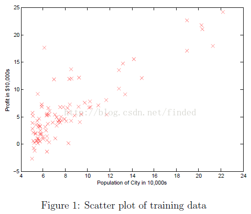
In thispart of this exercise, you will implement linear regression with one variableto predict profits for a food truck. Suppose you are the CEO of a restaurant franchiseand are considering different cities for opening a new outlet. The chainalready has trucks in various cities and you have data for profits andpopulations from the cities.

You wouldlike to use this data to help you select which city to expand to next.

1.1  Plotting the Data

function plotData(x, y)
%PLOTDATA Plots the data points x and y into a new figure 
%   PLOTDATA(x,y) plots the data points and gives the figure axes labels of
%   population and profit.

% ====================== YOUR CODE HERE ======================
% Instructions: Plot the training data into a figure using the 
%               "figure" and "plot" commands. Set the axes labels using
%               the "xlabel" and "ylabel" commands. Assume the 
%               population and revenue data have been passed in
%               as the x and y arguments of this function.
%
% Hint: You can use the 'rx' option with plot to have the markers
%       appear as red crosses. Furthermore, you can make the
%       markers larger by using plot(..., 'rx', 'MarkerSize', 10);

% data = load('ex1data1.txt'); % read comma separated data
% X = data(:, 1); y = data(:, 2);
% m = length(y);
% figure; % open a new figure window

plot (x,y,'rx','MarkerSize',10);  
ylabel('Profit in $ 10,000s');
xlabel('Population of City in 10,000s');

% ============================================================

end

1.2  Gradient Descent

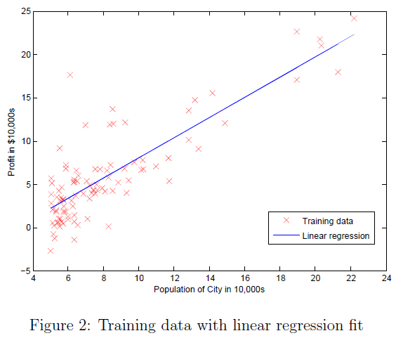
I will t the linear regression parameters to our dataset using gradient descent.

1.2.1 Update Equations

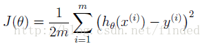
cost

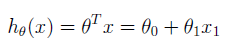
hypothesis

gradient descent

1.2.2 Implementation

2.2.3 Computing the cost J(theta)

<strong>function J = computeCost(X, y, theta)</strong>
%COMPUTECOST Compute cost for linear regression(Attention)

%   J = COMPUTECOST(X, y, theta) computes the cost of using theta as the
%   parameter for linear regression to fit the data points in X and y

% Initialize some useful values
m = length(y); % number of training examples, also m =size(X,1);

% You need to return the following variables correctly 
J = 0;


% ====================== YOUR CODE HERE ======================
% Instructions: Compute the cost of a particular choice of theta
%               You should set J to the cost.

m=size(X,1);                 % number of training examples m row X n colm
predictions=X*theta;         % predictions of hypothesis on all m examples
sqrErrors=(predictions-y).^2;% squared errors

J=1/(2*m)*sum(sqrErrors);    % cost function

% =========================================================================

end

1.2.4 Gradient descent

function [theta, J_history] = gradientDescent(X, y, theta, alpha, num_iters)
%GRADIENTDESCENT Performs gradient descent to learn theta
%   theta = GRADIENTDESENT(X, y, theta, alpha, num_iters) updates theta by 
%   taking num_iters gradient steps with learning rate alpha

% Initialize some useful values
m = length(y); % number of training examples
J_history = zeros(num_iters, 1);

%%%%%%%%%%%%%%%%%
n=length(X(1,:)); % number of features(include X0)
%initialize  vals to a matrix of 0's
%theta=zeros(size(X(1,:)'));
delta=zeros(n,1);

for iter = 1:num_iters

    % ====================== YOUR CODE HERE ======================
    % Instructions: Perform a single gradient step on the parameter vector
    %               theta. 
    %
    % Hint: While debugging, it can be useful to print out the values
    %       of the cost function (computeCost) and gradient here.
    %
 
predictions=X*theta;         % predictions of hypothesis on all m examples
errors=(predictions-y);      %  errors
sums=X'*errors;              %
delta=1/m *sums;

theta=theta-alpha*delta;     %iteration

    % ============================================================

    % Save the cost J in every iteration    
    J_history(iter) = computeCost(X, y, theta);

end

end

1.3  Debugging

1.4  Visualizing J(theta)

%% Machine Learning Online Class - Exercise 1: Linear Regression

%  Instructions
%  ------------
% 
%  This file contains code that helps you get started on the
%  linear exercise. You will need to complete the following functions 
%  in this exericse:
%
%     warmUpExercise.m
%     plotData.m
%     gradientDescent.m
%     computeCost.m
%     gradientDescentMulti.m
%     computeCostMulti.m
%     featureNormalize.m
%     normalEqn.m
%
%  For this exercise, you will not need to change any code in this file,
%  or any other files other than those mentioned above.
%
% x refers to the population size in 10,000s
% y refers to the profit in $10,000s
%

%% Initialization
clear ; close all; clc

%% ==================== Part 1: Basic Function ====================
% Complete warmUpExercise.m 
fprintf('Running warmUpExercise ... \n');
fprintf('5x5 Identity Matrix: \n');
warmUpExercise()

fprintf('Program paused. Press enter to continue.\n');
pause;


%% ======================= Part 2: Plotting =======================
fprintf('Plotting Data ...\n')
data = load('ex1data1.txt');
X = data(:, 1); y = data(:, 2);%只有一个变量，
m = length(y); % number of training examples

% Plot Data
% Note: You have to complete the code in plotData.m
plotData(X, y);

fprintf('Program paused. Press enter to continue.\n');
pause;

%% =================== Part 3: Gradient descent ===================
fprintf('Running Gradient Descent ...\n')

X = [ones(m, 1), data(:,1)]; % Add a column of ones to x
theta = zeros(2, 1); % initialize fitting parameters

% Some gradient descent settings
iterations = 1500;
alpha = 0.01;

% compute and display initial cost
computeCost(X, y, theta)

% run gradient descent
theta = gradientDescent(X, y, theta, alpha, iterations);

% print theta to screen
fprintf('Theta found by gradient descent: ');
fprintf('%f %f \n', theta(1), theta(2));

% Plot the linear fit
hold on; % keep previous plot visible
plot(X(:,2), X*theta, '-')
legend('Training data', 'Linear regression')
hold off % don't overlay any more plots on this figure

% Predict values for population sizes of 35,000 and 70,000
predict1 = [1, 3.5] *theta;
fprintf('For population = 35,000, we predict a profit of %f\n',...
    predict1*10000);
predict2 = [1, 7] * theta;
fprintf('For population = 70,000, we predict a profit of %f\n',...
    predict2*10000);

fprintf('Program paused. Press enter to continue.\n');
pause;

%% ============= Part 4: Visualizing J(theta_0, theta_1) =============
fprintf('Visualizing J(theta_0, theta_1) ...\n')

% Grid over which we will calculate J
theta0_vals = linspace(-10, 10, 100);
theta1_vals = linspace(-1, 4, 100);

% initialize J_vals to a matrix of 0's
J_vals = zeros(length(theta0_vals), length(theta1_vals));

% Fill out J_vals
for i = 1:length(theta0_vals)
    for j = 1:length(theta1_vals)
	  t = [theta0_vals(i); theta1_vals(j)];    
	  J_vals(i,j) = computeCost(X, y, t);
    end
end


% Because of the way meshgrids work in the surf command, we need to 
% transpose J_vals before calling surf, or else the axes will be flipped
J_vals = J_vals';
% Surface plot
figure;
surf(theta0_vals, theta1_vals, J_vals)
xlabel('\theta_0'); ylabel('\theta_1');

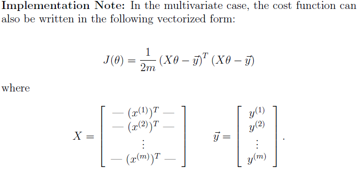
% Contour plot
figure;
% Plot J_vals as 15 contours spaced logarithmically between 0.01 and 100
contour(theta0_vals, theta1_vals, J_vals, logspace(-2, 3, 20))
xlabel('\theta_0'); ylabel('\theta_1');
hold on;
plot(theta(1), theta(2), 'rx', 'MarkerSize', 10, 'LineWidth', 2);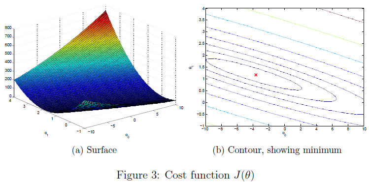

2   Linear regression with multiple variables

you will implement linear regression with multiple variables to predict the prices of houses. Suppose you are selling your house and you want to know what a good market price would be. One way to do this is to first collect information on recent houses sold and make a model of housing prices.

2.1  Feature Normalization

By looking at the values, note that house sizes are about 1000 times the number of bedrooms. When features diff er by orders of magnitude, first performing feature scaling can make gradient descent converge much more quickly.
Your task here is to complete the code in featureNormalize.m to
• Subtract the mean value of each feature from the dataset.
• After subtracting the mean, additionally scale (divide) the feature values by their respective \standard deviations."

function [X_norm, mu, sigma] = featureNormalize(X)
%FEATURENORMALIZE Normalizes the features in X 
%   FEATURENORMALIZE(X) returns a normalized version of X where
%   the mean value of each feature is 0 and the standard deviation
%   is 1. This is often a good preprocessing step to do when
%   working with learning algorithms.

% You need to set these values correctly
X_norm = X;
mu = zeros(1, size(X, 2));     % 1 x n
sigma = zeros(1, size(X, 2));  %1 x n


n= size(X,2); % n
m=size(X,1);
% ====================== YOUR CODE HERE ======================
% Instructions: First, for each feature dimension, compute the mean
%               of the feature and subtract it from the dataset,
%               storing the mean value in mu. Next, compute the 
%               standard deviation of each feature and divide
%               each feature by it's standard deviation, storing
%               the standard deviation in sigma. 
%
%               Note that X is a matrix where each column is a 
%               feature and each row is an example. You need 
%               to perform the normalization separately for 
%               each feature. 
%
% Hint: You might find the 'mean' and 'std' functions useful.
%       

mu=mean(X);   % 1 x n;
sigma=std(X) ;% 1 x n;

mu_temp=((mu')*ones(1,m))';  % m x n
sigma_temp=(sigma'*ones(1,m))' ; % m x n

X_norm=(X-mu_temp)./sigma_temp;

% ============================================================

end

2.2  Gradient Descent
Previously, you implemented gradient descent on a univariate regression problem. The only di fference now is that there is one more feature in the matrix X.

I complete the code in computeCostMulti.m and gradientDescentMulti.m to implement the cost function and gradient descent for linear regression with multiple variables.

cost functions with multiple various

function J = computeCostMulti(X, y, theta)
%COMPUTECOSTMULTI Compute cost for linear regression with multiple variables
%   J = COMPUTECOSTMULTI(X, y, theta) computes the cost of using theta as the
%   parameter for linear regression to fit the data points in X and y

% Initialize some useful values
m = length(y); % number of training examples

% You need to return the following variables correctly 
J = 0;

% ====================== YOUR CODE HERE ======================
% Instructions: Compute the cost of a particular choice of theta
%               You should set J to the cost.
m=size(X,1);                 % number of training examples m row X n colm
predictions=X*theta;         % predictions of hypothesis on all m examples
errors=predictions-y;% squared errors

J=1/(2*m)*(errors)'*errors;    % cost function

% =========================================================================

end

gradien  functions with multiple various

function [theta, J_history] = gradientDescentMulti(X, y, theta, alpha, num_iters)
%GRADIENTDESCENTMULTI Performs gradient descent to learn theta
%   theta = GRADIENTDESCENTMULTI(x, y, theta, alpha, num_iters) updates theta by
%   taking num_iters gradient steps with learning rate alpha
% 好像和单变量的一样
% Initialize some useful values
m = length(y); % number of training examples
J_history = zeros(num_iters, 1);

%%%%%%%%%%%%%%%%%%%%%%%%
n= size(X,2);

%theta=zeros(n,1);
delta= zeros(n);

for iter = 1:num_iters

    % ====================== YOUR CODE HERE ======================
    % Instructions: Perform a single gradient step on the parameter vector
    %               theta. 
    %
    % Hint: While debugging, it can be useful to print out the values
    %       of the cost function (computeCostMulti) and gradient here.
    %

predictions=X*theta;         % predictions of hypothesis on all m examples
errors=(predictions-y);      %  errors
sums=X'*errors;              %
delta=1/m *sums;

theta=theta-alpha*delta;     %iteration

    % ============================================================

    % Save the cost J in every iteration    
    J_history(iter) = computeCostMulti(X, y, theta);

end

end

2.2.1  Optional (ungraded) exercise: Selecting learning rates

 Trying values of the learning rate on a log-scale, at multiplicative steps of about 3 times the previous value (i.e., 0.3, 0.1, 0.03, 0.01 and so on).

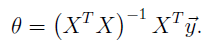
2.3  Normal Equations

The closed-form solution to linear regression is

function [X_norm, mu, sigma] = featureNormalize(X)
%FEATURENORMALIZE Normalizes the features in X 
%   FEATURENORMALIZE(X) returns a normalized version of X where
%   the mean value of each feature is 0 and the standard deviation
%   is 1. This is often a good preprocessing step to do when
%   working with learning algorithms.

% You need to set these values correctly
X_norm = X;
mu = zeros(1, size(X, 2));     % 1 x n
sigma = zeros(1, size(X, 2));  %1 x n


n= size(X,2); % n
m=size(X,1);
% ====================== YOUR CODE HERE ======================
% Instructions: First, for each feature dimension, compute the mean
%               of the feature and subtract it from the dataset,
%               storing the mean value in mu. Next, compute the 
%               standard deviation of each feature and divide
%               each feature by it's standard deviation, storing
%               the standard deviation in sigma. 
%
%               Note that X is a matrix where each column is a 
%               feature and each row is an example. You need 
%               to perform the normalization separately for 
%               each feature. 
%
% Hint: You might find the 'mean' and 'std' functions useful.
%       

mu=mean(X);   % 1 x n;
sigma=std(X) ;% 1 x n;

mu_temp=((mu')*ones(1,m))';  % m x n
sigma_temp=(sigma'*ones(1,m))' ; % m x n

X_norm=(X-mu_temp)./sigma_temp;

% ============================================================

end

Linear regression with multiple variables

%% Machine Learning Online Class
%  Exercise 1: Linear regression with multiple variables
%
%  Instructions
%  ------------
% 
%  This file contains code that helps you get started on the
%  linear regression exercise. 
%
%  You will need to complete the following functions in this 
%  exericse:
%
%     warmUpExercise.m
%     plotData.m
%     gradientDescent.m
%     computeCost.m
%     gradientDescentMulti.m
%     computeCostMulti.m
%     featureNormalize.m
%     normalEqn.m
%
%  For this part of the exercise, you will need to change some
%  parts of the code below for various experiments (e.g., changing
%  learning rates).
%

%% Initialization

%% ================ Part 1: Feature Normalization ================

%% Clear and Close Figures
clear ; close all; clc

fprintf('Loading data ...\n');

%% Load Data
data = load('ex1data2.txt');
X = data(:, 1:2);         % 两个变量
y = data(:, 3);
m = length(y);

% Print out some data points
fprintf('First 10 examples from the dataset: \n');
fprintf(' x = [%.0f %.0f], y = %.0f \n', [X(1:10,:) y(1:10,:)]');

fprintf('Program paused. Press enter to continue.\n');
pause;

% Scale features and set them to zero mean
fprintf('Normalizing Features ...\n');

[X mu sigma] = featureNormalize(X);%还没有添加X0那一列。fprintf('%.0f \n',X);

%fprintf(' x = [%.0f %.0f]\n', [X(1:10,:)]');
% Add intercept term to X
X = [ones(m, 1) X];





%% ================ Part 2: Gradient Descent ================

% ====================== YOUR CODE HERE ======================
% Instructions: We have provided you with the following starter
%               code that runs gradient descent with a particular
%               learning rate (alpha). 
%
%               Your task is to first make sure that your functions - 
%               computeCost and gradientDescent already work with 
%               this starter code and support multiple variables.
%
%               After that, try running gradient descent with 
%               different values of alpha and see which one gives
%               you the best result.
%
%               Finally, you should complete the code at the end
%               to predict the price of a 1650 sq-ft, 3 br house.
%
% Hint: By using the 'hold on' command, you can plot multiple
%       graphs on the same figure.
%
% Hint: At predictio  n, make sure you do the same feature normalization.
%

fprintf('Running gradient descent ...\n');



% Choose some alpha value
alpha = 1;     %i.e., 0.3, 0.1, 0.03, 0.01 and so on； default 0.01

num_iters = 400;  


% Init Theta and Run Gradient Descent 
theta = zeros(3, 1);
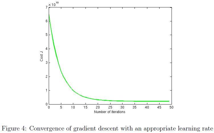
[theta, J_history] = gradientDescentMulti(X, y, theta, alpha, num_iters);

% Plot the convergence graph
figure;
plot(1:numel(J_history), J_history, '-b', 'LineWidth', 2);% num of elems
xlabel('Number of iterations');
ylabel('Cost J');

% Display gradient descent's result
fprintf('Theta computed from gradient descent: \n');
fprintf(' %f \n', theta);
fprintf('\n');


%%%%%%%%%%%%%%%%%%%%%%%%%%%%%%%%
% Init Theta and Run Gradient Descent 
% hold on;
% alpha1 = 0.003;
% theta1 = zeros(3, 1);
% alpha2 = 0.03;
% theta2 = zeros(3, 1);
% alpha3 = 0.1;
% theta3 = zeros(3, 1);
% alpha4 = 0.3;
% theta4 = zeros(3, 1);
% alpha5 = 1; %the best alpha
% theta5 = zeros(3, 1);
% [theta1, J_history1] = gradientDescentMulti(X, y, theta1, alpha1, num_iters);
% [theta2, J_history2] = gradientDescentMulti(X, y, theta2, alpha2, num_iters);
% [theta3, J_history3] = gradientDescentMulti(X, y, theta3, alpha3, num_iters);
% [theta4, J_history4] = gradientDescentMulti(X, y, theta4, alpha4, num_iters);
% [theta5, J_history5] = gradientDescentMulti(X, y, theta5, alpha5, num_iters)
% Plot the convergence graph
% plot(1:numel(J_history1), J_history1, '-r', 'LineWidth', 2);% num of elems
% hold on;
% plot(1:numel(J_history2), J_history2, '-y', 'LineWidth', 2);% num of elems
% hold on;
% plot(1:numel(J_history3), J_history3, '-g', 'LineWidth', 2);% num of elems
% hold on;
% plot(1:numel(J_history4), J_history4, '-y', 'LineWidth', 2);% num of elems
% hold on;
% plot(1:numel(J_history5), J_history5, '-r', 'LineWidth', 2);% num of elems
%%%%%%%%%%%%%%%%%%%%%%%%%%%%%%%%%%%%%%%%%%%%%%






% Estimate the price of a 1650 sq-ft, 3 br house
% ====================== YOUR CODE HERE ======================
% Recall that the first column of X is all-ones. Thus, it does
% not need to be normalized.
price = 0; % You should change this

x1=[1650,3];
 x1
x1=(x1.-mu)./sigma;
x1= [1,x1];
theta;
price=x1*theta;


% ============================================================

fprintf(['Predicted price of a 1650 sq-ft, 3 br house ' ...
         '(using gradient descent):\n $%f\n'], price);

fprintf('Program paused. Press enter to continue.\n');
pause;



%% ================ Part 3: Normal Equations ================

fprintf('Solving with normal equations...\n');

% ====================== YOUR CODE HERE ======================
% Instructions: The following code computes the closed form 
%               solution for linear regression using the normal
%               equations. You should complete the code in 
%               normalEqn.m
%
%               After doing so, you should complete this code 
%               to predict the price of a 1650 sq-ft, 3 br house.
%

%% Load Data
data = csvread('ex1data2.txt');
X = data(:, 1:2);
y = data(:, 3);
m = length(y);

% Add intercept term to X
X = [ones(m, 1) X];

% Calculate the parameters from the normal equation
theta = normalEqn(X, y);

% Display normal equation's result
fprintf('Theta computed from the normal equations: \n');
fprintf(' %f \n', theta);
fprintf('\n');


% Estimate the price of a 1650 sq-ft, 3 br house
% ====================== YOUR CODE HERE ======================
price = 0; % You should change this
price = 0; % You should change this
x1=[1,1650,3];
theta;
price=x1*theta;

% ============================================================

fprintf(['Predicted price of a 1650 sq-ft, 3 br house ' ...
         '(using normal equations):\n $%f\n'], price);