


This chapter covers
• The k-Nearest Neighbors classification algorithm
• Parsing and importing data from a text file• Creating scatter plots with Matplotlib
• Normalizing numeric values
1. The k-Nearest Neighbors classification algorithm
1). Brief Description
给定训练数据样本和标签,对于某测试的一个样本数据,选择距离其最近的k个训练样本,这k个训练样本中所属类别最多的类即为该测试样本的预测标签。
2). General approach to kNN
-
Collect: Any method.
-
Prepare: Numeric values are needed for a distance calculation. A structured dataformat is best.
-
Analyze: Any method.
-
Train: Does not apply to the kNN algorithm.
-
Test: Calculate the error rate.
-
Use: This application needs to get some input data and output structured num-eric values. Next, the application runs the kNN algorithm on this input data anddetermines which class the input data should belong to. The application thentakes some action on the calculated class.
'''
Created on Sep 16, 2010
kNN: k Nearest Neighbors

Input:      inX: vector to compare to existing dataset (1xN)
            dataSet: size m data set of known vectors (NxM)
            labels: data set labels (1xM vector)
            k: number of neighbors to use for comparison (should be an odd number)

Output:     the most popular class label

@author: pbharrin
'''

from numpy import *
from os import listdir
import operator


def createDataSet():  # 创建DataSet的一个范例
    group = array([[1.0, 1.1], [1.0, 1.0], [0, 0], [0, 0.1]])
    labels = ['A', 'A', 'B', 'B']
return group, labelscalculate the distance between inX and the current point
sort the distances in increasing order
take k items with lowest distances to inX
find the majority class among these items
return the majority class as our prediction for the class of inX
def classify0(inX, dataSet, labels, k):  # kNN classifier 简单K近邻算法
    dataSetSize = dataSet.shape[0]  # get 矩阵行数
    # tile函数:inX的第一维度重复dataSetSize遍,第二维度重复1遍
    diffMat = tile(inX, (dataSetSize, 1)) - dataSet
    sqDiffMat = diffMat ** 2  # squired different matrix
    sqDistances = sqDiffMat.sum(axis=1)  # sum函数:axis = 1 将矩阵每一行向量相加
    '''
    c = np.array([[0, 2, 1], [3, 5, 6], [0, 1, 1]])
    print c.sum()
    print c.sum(axis=0)
    print c.sum(axis=1)
    结果分别是:19, [3 8 8], [ 3 14  2]
    axis=0, 表示列。
    axis=1, 表示行。
    '''
    distances = sqDistances ** 0.5
    sortedDistIndicies = distances.argsort()  # argsort函数:返回的是数组值从小到大的indice
    classCount = {}
    for i in range(k):  # 选择距离最小的k个点
        voteIlabel = labels[sortedDistIndicies[i]]
        # get函数:在classCount中寻找voterIleabel的值, 如果不存在则返回0
        classCount[voteIlabel] = classCount.get(voteIlabel, 0) + 1
    sortedClassCount = sorted(classCount.items(),
                              key=operator.itemgetter(1),
                              reverse=True)
    '''
    排序函数sorted可以对list或者iterator进行排序
    iteritems():迭代输出dict的键值对,返回的是迭代器
    key为函数,指定取待排序元素的哪一项进行排序. operator.itemgetter(1)为根据第二个域进行排序
    reverse = true 降序排列
    '''
return sortedClassCount[0][0] # return the label of the item occuring most frequentlydef file2matrix(filename): # parse line to list
fr = open(filename)
numberOfLines = len(fr.readlines()) # get number of lines in file
# zeros函数:create Numpy matrix numberOfLines rows and 3 columns to return
returnMat = zeros((numberOfLines, 3))
classLabelVector = [] # to create an empty vector; prepare labels return
fr = open(filename)
index = 0
for line in fr.readlines():
line = line.strip() # strip函数:移除字符串头尾的指定字符(默认为空格)
# 对于每一行,按照制表符切割字符串,得到的结果构成一个数组,数组的每个元素代表一行中的一列;
# split the line into a list of elements delimited by the teb character'\t'
listFromLine = line.split('\t')
# parse line to a list;
# take the first three elements and shove them into a row of your
# matrix
returnMat[index, :] = listFromLine[0:3]
# get the last item from the list to put into classLabelVector
classLabelVector.append(int(listFromLine[-1]))
index += 1
return returnMat, classLabelVectordef img2vector(filename):
returnVect = zeros((1, 1024)) # 1 row, 1024 columns
fr = open(filename)
for i in range(32): # loop for row
lineStr = fr.readline() # 读取一行数字 数据类型?
for j in range(32): # loop for column
returnVect[0, 32*i+j] = int(lineStr[j])
return returnVect>>> import matplotlib
>>> import matplotlib.pyplot as plt
>>> fig = plt.figure()
>>> ax = fig.add_subplot(111)
>>> ax.scatter(datingDataMat[:,1], datingDataMat[:,2])
>>> plt.show()
>>> from numpy import *
>>> ax.scatter(datingDataMat[:,1], datingDataMat[:,2],
15.0*array(datingLabels), 15.0*array(datingLabels))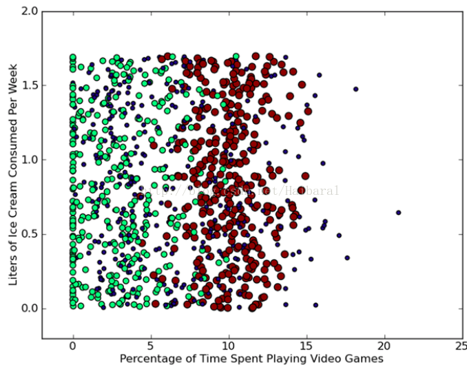
def autoNorm(dataSet): # Normalizing numeric values
# The 0 in dataSet.min(0) allows you to take the minimums from the
# columns, not the rows
minVals = dataSet.min(0)
maxVals = dataSet.max(0)
ranges = maxVals - minVals # max - min
normDataSet = zeros(shape(dataSet)) # shape(dataSet)获取矩阵的两个维度
m = dataSet.shape[0] # 行数
normDataSet = dataSet - tile(minVals, (m, 1)) # oldValue - min
# (oldValue - min)/(max - min) # element wise divide
normDataSet = normDataSet/tile(ranges, (m, 1))
return normDataSet, ranges, minValsdef datingClassTest(): # classifier testing code for dating site
hoRatio = 0.10
datingDataMat, datingLabels = file2matrix('datingTestSet2.txt')
normMat, ranges, minVals = autoNorm(datingDataMat)
m = normMat.shape[0] # 得到total number of data points
numTestVecs = int(m*hoRatio) # 用于测试的data number
errorCount = 0.0
for i in range(numTestVecs): # 将每个测试数据的结果与真实值相比较
classifierResult = classify0(normMat[i, :], normMat[numTestVecs:m, :],
datingLabels[numTestVecs:m], 3)
print("the classifier came back with: %d, the real answer is: %d" %
(classifierResult, datingLabels[i]))
if(classifierResult != datingLabels[i]):
errorCount += 1.0
print("the total error rate is: %f" % (errorCount/float(numTestVecs)))Prepare: Parse a text file in Python.
Analyze: Use Matplotlib to make 2D plots of our data.
Train: Doesn’t apply to the kNN algorithm.
Test: Write a function to use some portion of the data Hellen gave us as test ex- amples. The test examples are classified against the non-test examples. If the predicted class doesn’t match the real class, we’ll count that as an error.
Use: Build a simple command-line program Hellen can use to predict whether she’ll like someone based on a few inputs.
>>> reload(kNN)
>>> datingDataMat,datingLabels = kNN.file2matrix('datingTestSet.txt')
>>> datingDataMat
array([[ 7.29170000e+04, 7.10627300e+00, 2.23600000e-01],
[ 1.42830000e+04, 2.44186700e+00, 1.90838000e-01],
[ 7.34750000e+04, 8.31018900e+00, 8.52795000e-01],
...,
[ 1.24290000e+04, 4.43233100e+00, 9.24649000e-01],
[ 2.52880000e+04, 1.31899030e+01, 1.05013800e+00],
[ 4.91800000e+03, 3.01112400e+00, 1.90663000e-01]])
>>> datingLabels[0:20]
['didntLike', 'smallDoses', 'didntLike', 'largeDoses', 'smallDoses',
'smallDoses', 'didntLike', 'smallDoses', 'didntLike', 'didntLike', 'largeDoses', 'largeDose s', 'largeDoses', 'didntLike', 'didntLike', 'smallDoses', 'smallDoses', 'didntLike', 'smallDoses', 'didntLike']
>>> reload(kNN)
>>> normMat, ranges, minVals = kNN.autoNorm(datingDataMat)
>>> normMat
array([[ 0.33060119, 0.58918886, 0.69043973],
[ 0.49199139, 0.50262471, 0.13468257],
[ 0.34858782, 0.68886842, 0.59540619],
...,
[ 0.93077422, 0.52696233, 0.58885466],
[ 0.76626481, 0.44109859, 0.88192528],
[ 0.0975718 , 0.02096883, 0.02443895]])
>>> ranges
array([ 8.78430000e+04, 2.02823930e+01, 1.69197100e+00])
>>> minVals
array([ 0. , 0. , 0.001818])>>> kNN.datingClassTest()
the classifier came back with: 1, the real answer is: 1
the classifier came back with: 2, the real answer is: 2
.
.
the classifier came back with: 1, the real answer is: 1
the classifier came back with: 2, the real answer is: 2
the classifier came back with: 3, the real answer is: 3
the classifier came back with: 3, the real answer is: 1
the classifier came back with: 2, the real answer is: 2
the total error rate is: 0.024000def classifyPerson():
resultList = ['not at all', 'in small dosed', 'in large doses']
percentTats = float(input("percentage of time spent playing video games?"))
ffMiles = float(input("frequent flier miles earned per year?"))
iceCream = float(input("liters of ice cream consumed per year?"))
datingDataMat, datingLabels = file2matrix('datingTestSet2.txt')
normMat, ranges, minVals = autoNorm(datingDataMat)
inArr = array([ffMiles, percentTats, iceCream])
classifierResult = classify0(
(inArr-minVals)/ranges, normMat, datingLabels, 3)
print("You will probably like this person: ",
resultList[classifierResult - 1])>>> kNN.classifyPerson()
percentage of time spent playing video games?10
frequent flier miles earned per year?10000
liters of ice cream consumed per year?0.5
You will probably like this person: in small dosesPrepare: Write a function to convert from the image format to the list format used in our classifier, classify0().
Analyze: We’ll look at the prepared data in the Python shell to make sure it’s correct.
Train: Doesn’t apply to the kNN algorithm.
Test: Write a function to use some portion of the data as test examples. The test examples are classified against the non-test examples. If the predicted class doesn’t match the real class, you’ll count that as an error.
Use: Not performed in this example. You could build a complete program to extract digits from an image, such a system used to sort the mail in the United States.
def img2vector(filename):
    returnVect = zeros((1, 1024))  # 1 row, 1024 columns
    fr = open(filename)
    for i in range(32):  # loop for row
        lineStr = fr.readline()  # 读取一行数字 数据类型?
        for j in range(32):  # loop for column
            returnVect[0, 32*i+j] = int(lineStr[j])
return returnVect>>> testVector = kNN.img2vector('testDigits/0_13.txt')
>>> testVector[0,0:31]
array([ 0., 0., 0., 0., 0., 0., 0., 0., 0., 0., 0., 0., 0.,
0., 1., 1., 1., 1., 0., 0., 0., 0., 0., 0., 0., 0.,
0., 0., 0., 0., 0.])
>>> testVector[0,32:63]
array([ 0., 0., 0., 0., 0., 0., 0., 0., 0., 0., 0., 0., 1.,
1., 1., 1., 1., 1., 1., 0., 0., 0., 0., 0., 0., 0.,
0., 0., 0., 0., 0.])2). Test: kNN on handwritten digits
def handwritingClassTest():
    hwLabels = []
    trainingFileList = listdir('digits/trainingDigits')  # return list containing the names of the directory
    m = len(trainingFileList)  # 训练集的文件数目
    trainingMat = zeros((m, 1024))  # 创建training matrix, with m行, 1024列(32*32)
    for i in range(m):  # 将m个训练文件的class number及contents存入label(hwLabels) and training matrix
        fileNameStr = trainingFileList[i]  # 第i个文件夹全名
        fileStr = fileNameStr.split('.')[0]  # 文件名
        classNumStr = int(fileStr.split('_')[0])  # class number
        hwLabels.append(classNumStr)  # 将class num存入hwlabels
        # 将第i个文件的内容存入trainingMat(training matrix)的第i行
        trainingMat[i, :] = img2vector('digits/trainingDigits/%s' % fileNameStr)
    testFileList = listdir('digits/testDigits')
    errorCount = 0.0
    mTest = len(testFileList)
    for i in range(mTest):
        # Next, you do something similar for all the files in the testDigits directory
        fileNameStr = testFileList[i]
        fileStr = fileNameStr.split('.')[0]
        classNumStr = int(fileStr.split('_')[0])
        # but instead of loading them into a matrix, you test each vector individually with classify0
        vectorUnderTest = img2vector('digits/testDigits/%s' % fileNameStr)
        classifierResult = classify0(vectorUnderTest, trainingMat, hwLabels, 3)
        print("the classifier came back with: %d, the real answer is: %d" %
              (classifierResult, classNumStr))
        if(classifierResult != classNumStr): errorCount += 1.0
    print("\nthe total number of errors is: %d" % errorCount)
print("\nthetotal error rate is: %f" % (errorCount/float(mTest)))>>> kNN.handwritingClassTest()
the classifier came back with: 0, the real answer is: 0
the classifier came back with: 0, the real answer is: 0
.
.
the classifier came back with: 7, the real answer is: 7
the classifier came back with: 7, the real answer is: 7
the classifier came back with: 8, the real answer is: 8
the classifier came back with: 8, the real answer is: 8
the classifier came back with: 8, the real answer is: 8
the classifier came back with: 6, the real answer is: 8
.
.
the classifier came back with: 9, the real answer is: 9
the total number of errors is: 11
the total error rate is: 0.011628An additional drawback is that kNN doesn’t give you any idea of the underlying structure of the data; you have no idea what an “average” or “exemplar” instance from each class looks like. In the next chapter, we’ll address this issue by exploring ways in which probability measurements can help you do classification.
>>> import numpy
>>> numpy.tile([0,0],5)#在列方向上重复[0,0]5次,默认行1次
array([0, 0, 0, 0, 0, 0, 0, 0, 0, 0])
>>> numpy.tile([0,0],(1,1))#在列方向上重复[0,0]1次,行1次
array([[0, 0]])
>>> numpy.tile([0,0],(2,1))#在列方向上重复[0,0]1次,行2次
array([[0, 0],
       [0, 0]])
>>> numpy.tile([0,0],(3,1))
array([[0, 0],
       [0, 0],
       [0, 0]])
>>> numpy.tile([0,0],(1,3))#在列方向上重复[0,0]3次,行1次
array([[0, 0, 0, 0, 0, 0]])
>>> numpy.tile([0,0],(2,3))<span style="font-family: Arial, Helvetica, sans-serif;">#在列方向上重复[0,0]3次,行2次</span>
array([[0, 0, 0, 0, 0, 0],
       [0, 0, 0, 0, 0, 0]])


 203
203

 被折叠的 条评论
为什么被折叠?
被折叠的 条评论
为什么被折叠?
 到【灌水乐园】发言


