[深度学习论文笔记][Image Classification] Deep Residual Learning for Image Recognition

He, Kaiming, et al. “Deep residual learning for image recognition.” arXiv preprint arXiv:1512.03385 (2015). [Citations: 525].

1 Is Learning Better Networks as Easy as Stacking More Layers?

[Vanishing/Exploding Gradients] This problem can be largely addressed by careful initialization and intermediate BN layers.
[Degradation Problem] With the network depth increasing, accuracy gets saturated and then degrades rapidly. And this is not caused by overfitting or vanishing gradient.
• Overly deep plain nets have higher training and testing error.
• Not all systems are similarly easy to optimize.

• The solvers might have difficulties in approximating identity mappings by multiple nonlinear layers.

2 Deep Residual Learning
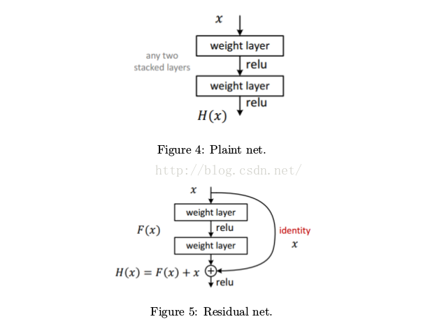
[Deep Residual Learning] Plaint net, see Fig. 4.
• H(x) is any desired mapping.
• Hope the 2 weight layers fit H(x) .
Residual net, see Fig. 5.
• H (x) is any desired mapping.
• Hope the 2 weight layers fit F(x) , such that H(x) = F(x) + x .
• If dimensions of x and F(x) are not equal, we can perform a linear projection W_P in the shortcut connections to match the dimensions.

3 Architecture

VGG style
• all 3 × 3 conv (with some 1 × 1 conv).
• When the feature map’s spatial size halved, the number of kernels is doubled.
• The downsampling is performed by conv with stride 2.
• BN is used after every conv layer.
• Dropout is not used since BN is adopted.

[In a Nutshell]
• Input (3 × 224 × 224).
• conv1 (64@7 × 7, s2), pool1 (3 × 3, s2).
• conv2x3.
• conv3x8.
• conv4x36.
• conv5x3, pool5 (global average pooling).
• fc6 (1000).

[Data Preparation (Training)] Resize the image whose shorter size is randomly sampled in U (256, 480) . Then the per-pixel mean is substracted.

[Data Augmentation (Training)] Random crop and its horizontal flip. And color augmentation.

[Data Augmentation (Training)] 10-crop testing. 

Adopt the fully-convolutional form and average the scores at multiple scales (images are resized such that the shorter side is in {224, 256, 384, 480, 640}).

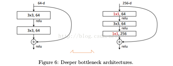
[Deeper Bottleneck Architectures] Use 1×1 conv to reduce and increase dimensions. See Fig. 6.

4 Training Details
SGD with momentum of 0.9
• Batch size 256.
• Weight decay 0.0001.
• Base learning rate 0.1.
• Training 600k iterations.
• Divide the learning rate by 10 when validation error plateaued.

5 Results
Winner of ILSVRC-2015.
• 1 CNN: 4.49%.
• 6 CNNs: 3.57%.

6 References
[1]. ICCV 2015. https://www.youtube.com/watch?v=1PGLj-uKT1w.