卡尔曼滤波之目标跟踪

本文目录：
1.关于卡尔曼滤波理论学习
2.卡尔曼滤波的两个简单使用示例
3. 卡尔曼滤波二维平面目标跟踪中的应用

1.关于卡尔曼滤波理论学习

之前的博文有关于 卡尔曼滤波的资料，通俗易懂。这里总结一下Kalman的公式精华，输入麻烦，直接上自己之前的笔记了，如下：

最最重要的一点，在使用卡尔曼滤波之前，首先你得弄清楚你假设的动态系统模型（说白了还是调参，跟pid一样），然后直接使用算法就行了。

2.卡尔曼滤波的两个简单python使用示例

jupyter notebook写的。

import numpy as np
import matplotlib.pyplot as plt
%matplotlib inline

例子一：单一的真实值在高斯噪声影响下的卡尔曼滤波

原地址：python起步之卡尔曼滤波

#这里是假设A=1，H=1的情况  

# intial parameters  
n_iter = 50  
sz = (n_iter,) # size of array  
x = -0.37727 # truth value (typo in example at top of p. 13 calls this z)  
z = np.random.normal(x,0.1,size=sz) # observations (normal about x, sigma=0.1)  

Q = 1e-5 # process variance  

# allocate space for arrays  
xhat=np.zeros(sz)      # a posteri estimate of x  
P=np.zeros(sz)         # a posteri error estimate  
xhatminus=np.zeros(sz) # a priori estimate of x  
Pminus=np.zeros(sz)    # a priori error estimate  
K=np.zeros(sz)         # gain or blending factor  

R = 0.1**2 # estimate of measurement variance, change to see effect 

# intial guesses  
xhat[0] = 0.0  
P[0] = 1.0  

for k in range(1,n_iter):  
    # time update  
    xhatminus[k] = xhat[k-1]  #X(k|k-1) = AX(k-1|k-1) + BU(k) + W(k),A=1,BU(k) = 0  
    Pminus[k] = P[k-1]+Q      #P(k|k-1) = AP(k-1|k-1)A' + Q(k) ,A=1  

    # measurement update  
    K[k] = Pminus[k]/( Pminus[k]+R ) #Kg(k)=P(k|k-1)H'/[HP(k|k-1)H' + R],H=1  
    xhat[k] = xhatminus[k]+K[k]*(z[k]-xhatminus[k]) #X(k|k) = X(k|k-1) + Kg(k)[Z(k) - HX(k|k-1)], H=1  
    P[k] = (1-K[k])*Pminus[k] #P(k|k) = (1 - Kg(k)H)P(k|k-1), H=1  

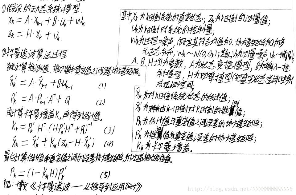
plt.figure()  
plt.plot(z,'k+',label='noisy measurements')     #测量值  
plt.plot(xhat,'b-',label='a posteri estimate')  #过滤后的值  
plt.axhline(x,color='g',label='truth value')    #系统值  
plt.legend()  
plt.xlabel('Iteration')  
plt.ylabel('Voltage')  

<matplotlib.text.Text at 0x7fe524000630>

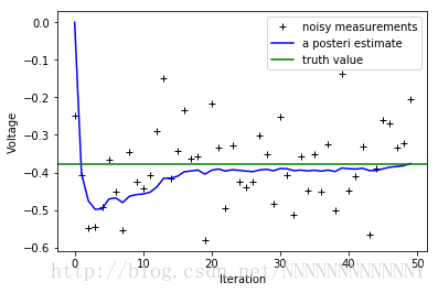
plt.figure()  
valid_iter = range(1,n_iter) # Pminus not valid at step 0  
plt.plot(valid_iter,Pminus[valid_iter],label='a priori error estimate')  
plt.xlabel('Iteration')  
plt.ylabel('$(Voltage)^2$')  
plt.setp(plt.gca(),'ylim',[0,.01])  
plt.show()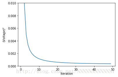  

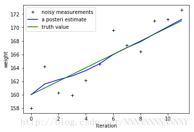
例子二：估计体重

原地址：【卡尔曼滤波器-Python】The g-h filter ， 有修改。

先大概看一下数据

z=np.array([158.0, 164.2, 160.3, 159.9, 162.1, 164.6, 169.6, 167.4, 166.4, 171.0, 171.2, 172.6]) 
x=np.arange(160, 172, 1) 
er=z-x 
plt.figure()
plt.scatter(er,np.zeros(12)) 
plt.show() 
print('mean:',np.mean(er)) 
print('var:',np.var(er))

mean: 0.108333333333
var: 4.50409722222

建立卡尔曼滤波的模型

$x_k=x_{k-1}+1$

$z_k=x_{k}+v_k$

总结：$A=1, B=1, u_k=1, w_k \sim N(0, 0)(即Q_k=0), H=1, v_k \sim N(0, 4.5)(即R_k=4.5)$

# intial parameters
z=np.array([158.0, 164.2, 160.3, 159.9, 162.1, 164.6, 169.6, 167.4, 166.4, 171.0, 171.2, 172.6]) 
A=1
B=1
u_k=1
Q=0
H=1
R=4.5
# allocate space for arrays  
sz=12
xhat=np.zeros(sz)      # a posteri estimate of x  
P=np.zeros(sz)         # a posteri error estimate  
xhatminus=np.zeros(sz) # a priori estimate of x  
Pminus=np.zeros(sz)    # a priori error estimate  
K=np.zeros(sz)         # gain or blending factor  

# intial guesses  
xhat[0] = 160 #设为真实值 
P[0] = 1.0  

for k in range(1,sz):  
    # time update  
    xhatminus[k] = A*xhat[k-1]+B*u_k  #X(k|k-1) = AX(k-1|k-1) + BU(k) + W(k),A=1,BU(k) = 0  
    Pminus[k] = A*P[k-1]*A+Q      #P(k|k-1) = AP(k-1|k-1)A' + Q(k) ,A=1  

    # measurement update  
    K[k] = Pminus[k]*H/(H*Pminus[k]*H + R ) #Kg(k)=P(k|k-1)H'/[HP(k|k-1)H' + R],H=1  
    xhat[k] = xhatminus[k]+K[k]*(z[k]-xhatminus[k]) #X(k|k) = X(k|k-1) + Kg(k)[Z(k) - HX(k|k-1)], H=1  
    P[k] = (1-K[k])*Pminus[k] #P(k|k) = (1 - Kg(k)H)P(k|k-1), H=1  

plt.figure()  
plt.plot(z,'k+',label='noisy measurements')     #测量值  
plt.plot(xhat,'b-',label='a posteri estimate')  #过滤后的值  
plt.plot(x,color='g',label='truth value')    #系统值  
plt.legend()  
plt.xlabel('Iteration')  
plt.ylabel('weight')  

<matplotlib.text.Text at 0x7fe52400aef0>

3. 卡尔曼滤波二维平面目标跟踪中的应用用

opencv官方给了个一维的示例，在opencv\sources\samples\cpp下，首先要把这个搞懂吧。
参见：opencv官方文档 cv::KalmanFilter::KalmanFilter ( )

好，现在卡尔曼滤波肯定已经搞明白了。但是图像处理中的目标跟踪，我的观测值从哪来？ 这句话简直太重要了，关于这个这的就因人而异了，卡尔曼滤波嘛，只是滤波而异，说白了是在最后一步对噪声的一个处理。至少我是这么想的，重点在于调参。
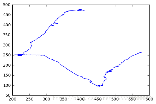
刚好最近做个东西用上二维下的目标跟踪，这里给个参考示例。
//加载数据，

import numpy as np
import matplotlib.pyplot as plt
%matplotlib inline

import re
tip_coordinate_re=re.compile(r'^(\d+):\s(\d+)\s(\d+)$')

tip_coordinate_x=[]
tip_coordinate_y=[]
with open('endPoint_estimation.txt') as f:
    for line in f.readlines():
        tip_coordinate_x.append(float(tip_coordinate_re.match(line.strip()).group(2)))
        tip_coordinate_y.append(float(tip_coordinate_re.match(line.strip()).group(3)))

plt.plot(tip_coordinate_x, tip_coordinate_y, '-')
plt.show()

（具体数据我这里就不给了，你可以用自己的或模拟一个）

//卡尔曼滤波

import numpy as np
import matplotlib.pyplot as plt

def kalman_xy(x, P, measurement, R,
              motion = np.matrix('0. 0. 0. 0.').T,
              Q = np.matrix(np.eye(4))):
    """
    Parameters:    
    x: initial state 4-tuple of location and velocity: (x0, x1, x0_dot, x1_dot)
    P: initial uncertainty convariance matrix
    measurement: observed position
    R: measurement noise 
    motion: external motion added to state vector x
    Q: motion noise (same shape as P)
    """
    return kalman(x, P, measurement, R, motion, Q,
                  F = np.matrix('''
                      1. 0. 1. 0.;
                      0. 1. 0. 1.;
                      0. 0. 1. 0.;
                      0. 0. 0. 1.
                      '''),
                  H = np.matrix('''
                      1. 0. 0. 0.;
                      0. 1. 0. 0.'''))

def kalman(x, P, measurement, R, motion, Q, F, H):
    '''
    Parameters:
    x: initial state
    P: initial uncertainty convariance matrix
    measurement: observed position (same shape as H*x)
    R: measurement noise (same shape as H)
    motion: external motion added to state vector x
    Q: motion noise (same shape as P)
    F: next state function: x_prime = F*x
    H: measurement function: position = H*x

    Return: the updated and predicted new values for (x, P)

    See also http://en.wikipedia.org/wiki/Kalman_filter

    This version of kalman can be applied to many different situations by
    appropriately defining F and H 
    '''
    # UPDATE x, P based on measurement m    
    # distance between measured and current position-belief
    y = np.matrix(measurement).T - H * x
    S = H * P * H.T + R  # residual convariance
    K = P * H.T * S.I    # Kalman gain
    x = x + K*y
    I = np.matrix(np.eye(F.shape[0])) # identity matrix
    P = (I - K*H)*P

    # PREDICT x, P based on motion
    x = F*x + motion
    P = F*P*F.T + Q

    return x, P

def demo_kalman_xy():
    x = np.matrix('0. 0. 0. 0.').T  #initial state 4-tuple of location and velocity
    P = np.matrix(np.eye(4))*1000 # initial uncertainty

#    N = 20
#    true_x = np.linspace(0.0, 10.0, N)
#    true_y = true_x**2
#    observed_x = true_x + 0.05*np.random.random(N)*true_x
#    observed_y = true_y + 0.05*np.random.random(N)*true_y
    observed_x = tip_coordinate_x
    observed_y = tip_coordinate_y
    plt.plot(observed_x, observed_y, 'ro')
    result = []
#    R = 0.01**2
    R = 0.01**2
    for meas in zip(observed_x, observed_y):
        x, P = kalman_xy(x, P, meas, R)
        result.append((x[:2]).tolist())
    kalman_x, kalman_y = zip(*result)
    plt.plot(kalman_x, kalman_y, 'g-')
    plt.show()

demo_kalman_xy()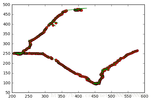

可以看到效果一般啦，具体还需要再调。
卡尔曼滤波部分的代码写得真好，声明不是本人所写，出自kalman 2d filter in python
。另外也可以参考下论文基于Kalman 预测的人体运动目标跟踪 。