Squeeze-and-Excitation Networks论文翻译——中英文对照

文章作者：Tyan
博客：noahsnail.com  |  CSDN  |  简书

声明：作者翻译论文仅为学习，如有侵权请联系作者删除博文，谢谢！

翻译论文汇总：https://github.com/SnailTyan/deep-learning-papers-translation

Squeeze-and-Excitation Networks

Abstract

Convolutional neural networks are built upon the convolution operation, which extracts informative features by fusing spatial and channel-wise information together within local receptive fields. In order to boost the representational power of a network, much existing work has shown the benefits of enhancing spatial encoding. In this work, we focus on channels and propose a novel architectural unit, which we term the “Squeeze-and-Excitation”(SE) block, that adaptively recalibrates channel-wise feature responses by explicitly modelling interdependencies between channels. We demonstrate that by stacking these blocks together, we can construct SENet architectures that generalise extremely well across challenging datasets. Crucially, we find that SE blocks produce significant performance improvements for existing state-of-the-art deep architectures at slight computational cost. SENets formed the foundation of our ILSVRC 2017 classification submission which won first place and significantly reduced the top-5 error to $2.251\%$, achieving a $\sim25\%$ relative improvement over the winning entry of 2016.

摘要

卷积神经网络建立在卷积运算的基础上，通过融合局部感受野内的空间信息和通道信息来提取信息特征。为了提高网络的表示能力，许多现有的工作已经显示出增强空间编码的好处。在这项工作中，我们专注于通道，并提出了一种新颖的架构单元，我们称之为“Squeeze-and-Excitation”（SE）块，通过显式地建模通道之间的相互依赖关系，自适应地重新校准通道式的特征响应。通过将这些块堆叠在一起，我们证明了我们可以构建SENet架构，在具有挑战性的数据集中可以进行泛化地非常好。关键的是，我们发现SE块以微小的计算成本为现有的最先进的深层架构产生了显著的性能改进。SENets是我们ILSVRC 2017分类提交的基础，它赢得了第一名，并将top-5错误率显著减少到$2.251 \%$，相对于2016年的获胜成绩取得了$\sim25\%$的相对改进。

1. Introduction

Convolutional neural networks (CNNs) have proven to be effective models for tackling a variety of visual tasks [19, 23, 29, 41]. For each convolutional layer, a set of filters are learned to express local spatial connectivity patterns along input channels. In other words, convolutional filters are expected to be informative combinations by fusing spatial and channel-wise information together, while restricted in local receptive fields. By stacking a series of convolutional layers interleaved with non-linearities and downsampling, CNNs are capable of capturing hierarchical patterns with global receptive fields as powerful image descriptions. Recent work has demonstrated the performance of networks can be improved by explicitly embedding learning mechanisms that help capture spatial correlations without requiring additional supervision. One such approach was popularised by the Inception architectures [14, 39], which showed that the network can achieve competitive accuracy by embedding multi-scale processes in its modules. More recent work has sought to better model spatial dependence [1, 27] and incorporate spatial attention [17].

1. 引言

卷积神经网络（CNNs）已被证明是解决各种视觉任务的有效模型[19,23,29,41]。对于每个卷积层，沿着输入通道学习一组滤波器来表达局部空间连接模式。换句话说，期望卷积滤波器通过融合空间信息和信道信息进行信息组合，而受限于局部感受野。通过叠加一系列非线性和下采样交织的卷积层，CNN能够捕获具有全局感受野的分层模式作为强大的图像描述。最近的工作已经证明，网络的性能可以通过显式地嵌入学习机制来改善，这种学习机制有助于捕捉空间相关性而不需要额外的监督。Inception架构推广了一种这样的方法[14,39]，这表明网络可以通过在其模块中嵌入多尺度处理来取得有竞争力的准确度。最近的工作在寻找更好地模型空间依赖[1,27]，结合空间注意力[17]。

In contrast to these methods, we investigate a different aspect of architectural design —— the channel relationship, by introducing a new architectural unit, which we term the “Squeeze-and-Excitation” (SE) block. Our goal is to improve the representational power of a network by explicitly modelling the interdependencies between the channels of its convolutional features. To achieve this, we propose a mechanism that allows the network to perform feature recalibration, through which it can learn to use global information to selectively emphasise informative features and suppress less useful ones.

与这些方法相反，通过引入新的架构单元，我们称之为“Squeeze-and-Excitation” (SE)块，我们研究了架构设计的一个不同方向——通道关系。我们的目标是通过显式地建模卷积特征通道之间的相互依赖性来提高网络的表示能力。为了达到这个目的，我们提出了一种机制，使网络能够执行特征重新校准，通过这种机制可以学习使用全局信息来选择性地强调信息特征并抑制不太有用的特征。

The basic structure of the SE building block is illustrated in Fig.1. For any given transformation $\mathbf{F}_{tr} : \mathbf{X} \rightarrow \mathbf{U}$, $\mathbf{X} \in \mathbb{R}^{W' \times H' \times C'}, \mathbf{U} \in \mathbb{R}^{W \times H \times C}$, (e.g. a convolution or a set of convolutions), we can construct a corresponding SE block to perform feature recalibration as follows. The features $\mathbf{U}$ are first passed through a squeeze operation, which aggregates the feature maps across spatial dimensions $W \times H$ to produce a channel descriptor. This descriptor embeds the global distribution of channel-wise feature responses, enabling information from the global receptive field of the network to be leveraged by its lower layers. This is followed by an excitation operation, in which sample-specific activations, learned for each channel by a self-gating mechanism based on channel dependence, govern the excitation of each channel. The feature maps $\mathbf{U}$ are then reweighted to generate the output of the SE block which can then be fed directly into subsequent layers.

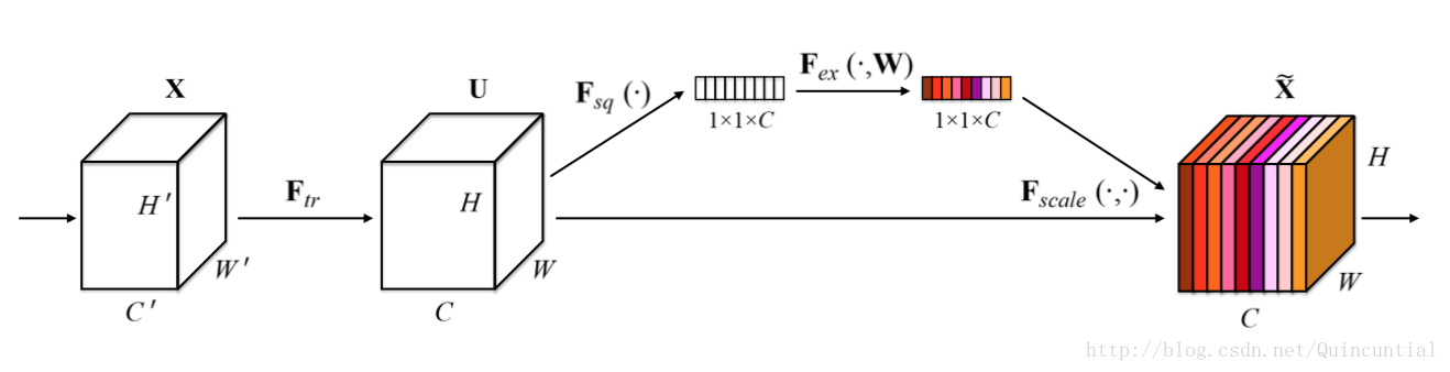
Figure 1. A Squeeze-and-Excitation block.

SE构建块的基本结构如图1所示。对于任何给定的变换$\mathbf{F}_{tr} : \mathbf{X} \rightarrow \mathbf{U}$, $\mathbf{X} \in \mathbb{R}^{W' \times H' \times C'}, \mathbf{U} \in \mathbb{R}^{W \times H \times C}$，(例如卷积或一组卷积)，我们可以构造一个相应的SE块来执行特征重新校准，如下所示。特征$\mathbf{U}$首先通过squeeze操作，该操作跨越空间维度$W \times H$聚合特征映射来产生通道描述符。这个描述符嵌入了通道特征响应的全局分布，使来自网络全局感受野的信息能够被其较低层利用。这之后是一个excitation操作，其中通过基于通道依赖性的自门机制为每个通道学习特定采样的激活，控制每个通道的激励。然后特征映射$\mathbf{U}$被重新加权以生成SE块的输出，然后可以将其直接输入到随后的层中。

图1. Squeeze-and-Excitation块

An SE network can be generated by simply stacking a collection of SE building blocks. SE blocks can also be used as a drop-in replacement for the original block at any depth in the architecture. However, while the template for the building block is generic, as we show in Sec. 6.3, the role it performs at different depths adapts to the needs of the network. In the early layers, it learns to excite informative features in a class agnostic manner, bolstering the quality of the shared lower level representations. In later layers, the SE block becomes increasingly specialised, and responds to different inputs in a highly class-specific manner. Consequently, the benefits of feature recalibration conducted by SE blocks can be accumulated through the entire network.

SE网络可以通过简单地堆叠SE构建块的集合来生成。SE块也可以用作架构中任意深度的原始块的直接替换。然而，虽然构建块的模板是通用的，正如我们6.3节中展示的那样，但它在不同深度的作用适应于网络的需求。在前面的层中，它学习以类不可知的方式激发信息特征，增强共享的较低层表示的质量。在后面的层中，SE块越来越专业化，并以高度类特定的方式响应不同的输入。因此，SE块进行特征重新校准的好处可以通过整个网络进行累积。

The development of new CNN architectures is a challenging engineering task, typically involving the selection of many new hyperparameters and layer configurations. By contrast, the design of the SE block outlined above is simple, and can be used directly with existing state-of-the-art architectures whose convolutional layers can be strengthened by direct replacement with their SE counterparts. Moreover, as shown in Sec. 4, SE blocks are computationally lightweight and impose only a slight increase in model complexity and computational burden. To support these claims, we develop several SENets, namely SE-ResNet, SE-Inception, SE-ResNeXt and SE-Inception-ResNet and provide an extensive evaluation of SENets on the ImageNet 2012 dataset [30]. Further, to demonstrate the general applicability of SE blocks, we also present results beyond ImageNet, indicating that the proposed approach is not restricted to a specific dataset or a task.

新CNN架构的开发是一项具有挑战性的工程任务，通常涉及许多新的超参数和层配置的选择。相比之下，上面概述的SE块的设计是简单的，并且可以直接与现有的最新架构一起使用，其卷积层可以通过直接用对应的SE层来替换从而进行加强。另外，如第四节所示，SE块在计算上是轻量级的，并且在模型复杂性和计算负担方面仅稍微增加。为了支持这些声明，我们开发了一些SENets，即SE-ResNet，SE-Inception，SE-ResNeXt和SE-Inception-ResNet，并在ImageNet 2012数据集[30]上对SENets进行了广泛的评估。此外，为了证明SE块的一般适用性，我们还呈现了ImageNet之外的结果，表明所提出的方法不受限于特定的数据集或任务。

Using SENets, we won the first place in the ILSVRC 2017 classification competition. Our top performing model ensemble achieves a $2.251\%$ top-5 error on the test set. This represents a $\sim 25\%$ relative improvement in comparison to the winner entry of the previous year (with a top-$5$ error of $2.991\%$). Our models and related materials have been made available to the research community.

使用SENets，我们赢得了ILSVRC 2017分类竞赛的第一名。我们的表现最好的模型集合在测试集上达到了$2.251\%$的top-5错误率。与前一年的获奖者（$2.991\%$的top-5错误率）相比，这表示$\sim 25\%$的相对改进。我们的模型和相关材料已经提供给研究界。

2. Related Work

Deep architectures. A wide range of work has shown that restructuring the architecture of a convolutional neural network in a manner that eases the learning of deep features can yield substantial improvements in performance. VGGNets [35] and Inception models [39] demonstrated the benefits that could be attained with an increased depth, significantly outperforming previous approaches on ILSVRC 2014. Batch normalization (BN) [14] improved gradient propagation through deep networks by inserting units to regulate layer inputs stabilising the learning process, which enables further experimentation with a greater depth. He et al. [9, 10] showed that it was effective to train deeper networks by restructuring the architecture to learn residual functions through the use of identity-based skip connections which ease the flow of information across units. More recently, reformulations of the connections between network layers [5, 12] have been shown to further improve the learning and representational properties of deep networks.

2. 近期工作

深层架构。大量的工作已经表明，以易于学习深度特征的方式重构卷积神经网络的架构可以大大提高性能。VGGNets[35]和Inception模型[39]证明了深度增加可以获得的好处，明显超过了ILSVRC 2014之前的方法。批标准化（BN）[14]通过插入单元来调节层输入稳定学习过程，改善了通过深度网络的梯度传播，这使得可以用更深的深度进行进一步的实验。He等人[9,10]表明，通过重构架构来训练更深层次的网络是有效的，通过使用基于恒等映射的跳跃连接来学习残差函数，从而减少跨单元的信息流动。最近，网络层间连接的重新表示[5,12]已被证明可以进一步改善深度网络的学习和表征属性。

An alternative line of research has explored ways to tune the functional form of the modular components of a network. Grouped convolutions can be used to increase cardinality (the size of the set of transformations) [13, 43] to learn richer representations. Multi-branch convolutions can be interpreted as a generalisation of this concept, enabling more flexible compositions of convolutional operators [14, 38, 39, 40]. Cross-channel correlations are typically mapped as new combinations of features, either independently of spatial structure [6, 18] or jointly by using standard convolutional filters [22] with $1\times 1$ convolutions, while much of this work has concentrated on the objective of reducing model and computational complexity. This approach reflects an assumption that channel relationships can be formulated as a composition of instance-agnostic functions with local receptive fields. In contrast, we claim that providing the network with a mechanism to explicitly model dynamic, non-linear dependencies between channels using global information can ease the learning process, and significantly enhance the representational power of the network.

另一种研究方法探索了调整网络模块化组件功能形式的方法。可以用分组卷积来增加基数（一组变换的大小）[13,43]以学习更丰富的表示。多分支卷积可以解释为这个概念的概括，使得卷积算子可以更灵活的组合[14,38,39,40]。跨通道相关性通常被映射为新的特征组合，或者独立的空间结构[6,18]，或者联合使用标准卷积滤波器[22]和$1\times 1$卷积，然而大部分工作的目标是集中在减少模型和计算复杂度上面。这种方法反映了一个假设，即通道关系可以被表述为具有局部感受野的实例不可知的函数的组合。相比之下，我们声称为网络提供一种机制来显式建模通道之间的动态、非线性依赖关系，使用全局信息可以减轻学习过程，并且显著增强网络的表示能力。

Attention and gating mechanisms. Attention can be viewed, broadly, as a tool to bias the allocation of available processing resources towards the most informative components of an input signal. The development and understanding of such mechanisms has been a longstanding area of research in the neuroscience community [15, 16, 28] and has seen significant interest in recent years as a powerful addition to deep neural networks [20, 25]. Attention has been shown to improve performance across a range of tasks, from localisation and understanding in images [3, 17] to sequence-based models [2, 24]. It is typically implemented in combination with a gating function (e.g. a softmax or sigmoid) and sequential techniques [11, 37]. Recent work has shown its applicability to tasks such as image captioning [4, 44] and lip reading [7], in which it is exploited to efficiently aggregate multi-modal data. In these applications, it is typically used on top of one or more layers representing higher-level abstractions for adaptation between modalities. Highway networks [36] employ a gating mechanism to regulate the shortcut connection, enabling the learning of very deep architectures. Wang et al. [42] introduce a powerful trunk-and-mask attention mechanism using an hourglass module [27], inspired by its success in semantic segmentation. This high capacity unit is inserted into deep residual networks between intermediate stages. In contrast, our proposed SE-block is a lightweight gating mechanism, specialised to model channel-wise relationships in a computationally efficient manner and designed to enhance the representational power of modules throughout the network.

注意力和门机制。从广义上讲，可以将注意力视为一种工具，将可用处理资源的分配偏向于输入信号的信息最丰富的组成部分。这种机制的发展和理解一直是神经科学社区的一个长期研究领域[15,16,28]，并且近年来作为一个强大补充，已经引起了深度神经网络的极大兴趣[20,25]。注意力已经被证明可以改善一系列任务的性能，从图像的定位和理解[3,17]到基于序列的模型[2,24]。它通常结合门功能（例如softmax或sigmoid）和序列技术来实现[11,37]。最近的研究表明，它适用于像图像标题[4,44]和口头阅读[7]等任务，其中利用它来有效地汇集多模态数据。在这些应用中，它通常用在表示较高级别抽象的一个或多个层的顶部，以用于模态之间的适应。高速网络[36]采用门机制来调节快捷连接，使得可以学习非常深的架构。王等人[42]受到语义分割成功的启发，引入了一个使用沙漏模块[27]的强大的trunk-and-mask注意力机制。这个高容量的单元被插入到中间阶段之间的深度残差网络中。相比之下，我们提出的SE块是一个轻量级的门机制，专门用于以计算有效的方式对通道关系进行建模，并设计用于增强整个网络中模块的表示能力。

3. Squeeze-and-Excitation Blocks

The Squeeze-and-Excitation block is a computational unit which can be constructed for any given transformation $\mathbf{F}_{tr}: \mathbf{X} \rightarrow \mathbf{U}, \, \mathbf{X} \in \mathbb{R}^{W' \times H' \times C'}, \mathbf{U} \in \mathbb{R}^{W \times H \times C}$. For simplicity of exposition, in the notation that follows we take $\mathbf{F}_{tr}$ to be a standard convolutional operator. Let $\mathbf{V}= [\mathbf{v}_1, \mathbf{v}_2, \dots, \mathbf{v}_{C}]$ denote the learned set of filter kernels, where $\mathbf{v}_c$ refers to the parameters of the $c$-th filter. We can then write the outputs of $\mathbf{F}_{tr}$ as $\mathbf{U} = [\mathbf{u}_1, \mathbf{u}_2, \dots, \mathbf{u}_{C}]$ where

$$\mathbf{u}_c = \mathbf{v}_c \ast \mathbf{X} = \sum_{s=1}^{C'}\mathbf{v}^s_c \ast \mathbf{x}^s.$$ Here $\ast$ denotes convolution, $\mathbf{v}_c = [\mathbf{v}^1_c, \mathbf{v}^2_c, \dots, \mathbf{v}^{C'}_c]$ and $\mathbf{X} = [\mathbf{x}^1, \mathbf{x}^2, \dots, \mathbf{x}^{C'}]$ (to simplify the notation, bias terms are omitted). Here $\mathbf{v}^s_c$ is a $2$D spatial kernel, and therefore represents a single channel of $\mathbf{v}_c$ which acts on the corresponding channel of $\mathbf{X}$. Since the output is produced by a summation through all channels, the channel dependencies are implicitly embedded in $\mathbf{v}_c$, but these dependencies are entangled with the spatial correlation captured by the filters. Our goal is to ensure that the network is able to increase its sensitivity to informative features so that they can be exploited by subsequent transformations, and to suppress less useful ones. We propose to achieve this by explicitly modelling channel interdependencies to recalibrate filter responses in two steps, squeeze and excitation, before they are fed into next transformation. A diagram of an SE building block is shown in Fig.1.

3. Squeeze-and-Excitation块

Squeeze-and-Excitation块是一个计算单元，可以为任何给定的变换构建：$\mathbf{F}_{tr}: \mathbf{X} \rightarrow \mathbf{U}, \, \mathbf{X} \in \mathbb{R}^{W' \times H' \times C'}, \mathbf{U} \in \mathbb{R}^{W \times H \times C}$。为了简化说明，在接下来的表示中，我们将$\mathbf{F}_{tr}$看作一个标准的卷积算子。$\mathbf{V}= [\mathbf{v}_1, \mathbf{v}_2, \dots, \mathbf{v}_{C}]$表示学习到的一组滤波器核，$\mathbf{v}_c$指的是第$c$个滤波器的参数。然后我们可以将$\mathbf{F}_{tr}$的输出写作$\mathbf{U} = [\mathbf{u}_1, \mathbf{u}_2, \dots, \mathbf{u}_{C}]$，其中

$$\mathbf{u}_c = \mathbf{v}_c \ast \mathbf{X} = \sum_{s=1}^{C'}\mathbf{v}^s_c \ast \mathbf{x}^s.$$ 这里 $\ast$表示卷积， $\mathbf{v}_c = [\mathbf{v}^1_c, \mathbf{v}^2_c, \dots, \mathbf{v}^{C'}_c]$， $\mathbf{X} = [\mathbf{x}^1, \mathbf{x}^2, \dots, \mathbf{x}^{C'}]$（为了简洁表示，忽略偏置项）。这里 $\mathbf{v}^s_c$是 $2$D空间核，因此表示$\mathbf{v}_c$的一个单通道，作用于对应的通道 $\mathbf{X}$。由于输出是通过所有通道的和来产生的，所以通道依赖性被隐式地嵌入到 $\mathbf{v}_c$中，但是这些依赖性与滤波器捕获的空间相关性纠缠在一起。我们的目标是确保能够提高网络对信息特征的敏感度，以便后续转换可以利用这些功能，并抑制不太有用的功能。我们建议通过显式建模通道依赖性来实现这一点，以便在进入下一个转换之前通过两步重新校准滤波器响应，两步为： squeeze和 excitation。SE构建块的图如图1所示。

3.1. Squeeze: Global Information Embedding

In order to tackle the issue of exploiting channel dependencies, we first consider the signal to each channel in the output features. Each of the learned filters operate with a local receptive field and consequently each unit of the transformation output $\mathbf{U}$ is unable to exploit contextual information outside of this region. This is an issue that becomes more severe in the lower layers of the network whose receptive field sizes are small.

3.1. Squeeze:全局信息嵌入

为了解决利用通道依赖性的问题，我们首先考虑输出特征中每个通道的信号。每个学习到的滤波器都对局部感受野进行操作，因此变换输出$\mathbf{U}$的每个单元都无法利用该区域之外的上下文信息。在网络较低的层次上其感受野尺寸很小，这个问题变得更严重。

To mitigate this problem, we propose to squeeze global spatial information into a channel descriptor. This is achieved by using global average pooling to generate channel-wise statistics. Formally, a statistic $\mathbf{z} \in \mathbb{R}^{C}$ is generated by shrinking $\mathbf{U}$ through spatial dimensions $W \times H$, where the $c$-th element of $\mathbf{z}$ is calculated by:

$$z_c = \mathbf{F}_{sq}(\mathbf{u}_c) = \frac{1}{W \times H}\sum_{i=1}^{W} \sum_{j=1}^{H} u_c(i,j).$$

为了减轻这个问题，我们提出将全局空间信息压缩成一个通道描述符。这是通过使用全局平均池化生成通道统计实现的。形式上，统计$\mathbf{z} \in \mathbb{R}^{C}$是通过在空间维度$W \times H$上收缩$\mathbf{U}$生成的，其中$\mathbf{z}$的第$c$个元素通过下式计算：

$$z_c = \mathbf{F}_{sq}(\mathbf{u}_c) = \frac{1}{W \times H}\sum_{i=1}^{W} \sum_{j=1}^{H} u_c(i,j).$$

Discussion. The transformation output $\mathbf{U}$ can be interpreted as a collection of the local descriptors whose statistics are expressive for the whole image. Exploiting such information is prevalent in feature engineering work [31, 34, 45]. We opt for the simplest, global average pooling, while more sophisticated aggregation strategies could be employed here as well.

讨论。转换输出$\mathbf{U}$可以被解释为局部描述子的集合，这些描述子的统计信息对于整个图像来说是有表现力的。特征工程工作中[31,34,45]普遍使用这些信息。我们选择最简单的全局平均池化，同时也可以采用更复杂的汇聚策略。

3.2. Excitation: Adaptive Recalibration

To make use of the information aggregated in the squeeze operation, we follow it with a second operation which aims to fully capture channel-wise dependencies. To fulfil this objective, the function must meet two criteria: first, it must be flexible (in particular, it must be capable of learning a nonlinear interaction between channels) and second, it must learn a non-mutually-exclusive relationship as multiple channels are allowed to be emphasised opposed to one-hot activation. To meet these criteria, we opt to employ a simple gating mechanism with a sigmoid activation:

$$\mathbf{s} = \mathbf{F}_{ex}(\mathbf{z}, \mathbf{W}) = \sigma(g(\mathbf{z}, \mathbf{W})) = \sigma(\mathbf{W}_2\delta(\mathbf{W}_1\mathbf{z}))$$ where $\delta$ refers to the ReLU[26] function, $\mathbf{W}_1 \in \mathbb{R}^{\frac{C}{r} \times C}$ and $\mathbf{W}_2 \in \mathbb{R}^{C \times \frac{C}{r}}$. To limit model complexity and aid generalisation, we parameterise the gating mechanism by forming a bottleneck with two fully-connected (FC) layers around the non-linearity, i.e. a dimensionality-reduction layer with parameters $\mathbf{W}_1$ with reduction ratio $r$ (we set it to be 16, and this parameter choice is discussed in Sec.6.3), a ReLU and then a dimensionality-increasing layer with parameters $\mathbf{W}_2$. The final output of the block is obtained by rescaling the transformation output $\mathbf{U}$ with the activations: $$\widetilde{\mathbf{x}}_c = \mathbf{F}_{scale}(\mathbf{u}_c, s_c) = s_c \cdot \mathbf{u}_c$$ where $\widetilde{\mathbf{X}} = [\widetilde{\mathbf{x}}_1, \widetilde{\mathbf{x}}_2, \dots, \widetilde{\mathbf{x}}_{C}]$ and $\mathbf{F}_{scale}(\mathbf{u}_c, s_c)$ refers to channel-wise multiplication between the feature map $\mathbf{u}_c \in \mathbb{R}^{W \times H}$ and the scalar $s_c$.

3.2. Excitation:自适应重新校正

为了利用压缩操作中汇聚的信息，我们接下来通过第二个操作来全面捕获通道依赖性。为了实现这个目标，这个功能必须符合两个标准：第一，它必须是灵活的（特别是它必须能够学习通道之间的非线性交互）；第二，它必须学习一个非互斥的关系，因为独热激活相反，这里允许强调多个通道。为了满足这些标准，我们选择采用一个简单的门机制，并使用sigmoid激活：

$$\mathbf{s} = \mathbf{F}_{ex}(\mathbf{z}, \mathbf{W}) = \sigma(g(\mathbf{z}, \mathbf{W})) = \sigma(\mathbf{W}_2\delta(\mathbf{W}_1\mathbf{z}))$$ ，其中 $\delta$是指ReLU[26]函数， $\mathbf{W}_1 \in \mathbb{R}^{\frac{C}{r} \times C}$和 $\mathbf{W}_2 \in \mathbb{R}^{C \times \frac{C}{r}}$。为了限制模型复杂度和辅助泛化，我们通过在非线性周围形成两个全连接（FC）层的瓶颈来参数化门机制，即降维层参数为 $\mathbf{W}_1$，降维比例为 $r$（我们把它设置为16，这个参数选择在6.3节中讨论），一个ReLU，然后是一个参数为$\mathbf{W}_2$的升维层。块的最终输出通过重新调节带有激活的变换输出 $\mathbf{U}$得到： $$\widetilde{\mathbf{x}}_c = \mathbf{F}_{scale}(\mathbf{u}_c, s_c) = s_c \cdot \mathbf{u}_c$$ 其中 $\widetilde{\mathbf{X}} = [\widetilde{\mathbf{x}}_1, \widetilde{\mathbf{x}}_2, \dots, \widetilde{\mathbf{x}}_{C}]$和 $\mathbf{F}_{scale}(\mathbf{u}_c, s_c)$指的是特征映射 $\mathbf{u}_c \in \mathbb{R}^{W \times H}$和标量 $s_c$之间的对应通道乘积。

Discussion. The activations act as channel weights adapted to the input-specific descriptor $\mathbf{z}$. In this regard, SE blocks intrinsically introduce dynamics conditioned on the input, helping to boost feature discriminability.

讨论。激活作为适应特定输入描述符$\mathbf{z}$的通道权重。在这方面，SE块本质上引入了以输入为条件的动态特性，有助于提高特征辨别力。

3.3. Exemplars: SE-Inception and SE-ResNet

The flexibility of the SE block means that it can be directly applied to transformations beyond standard convolutions. To illustrate this point, we develop SENets by integrating SE blocks into two popular network families of architectures, Inception and ResNet. SE blocks are constructed for the Inception network by taking the transformation $\mathbf{F}_{tr}$ to be an entire Inception module (see Fig.2). By making this change for each such module in the architecture, we construct an SE-Inception network.

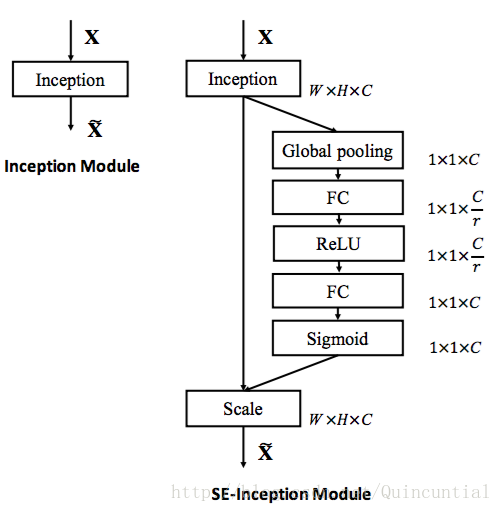
Figure 2. The schema of the original Inception module (left) and the SE-Inception module (right).

3.3. 模型：SE-Inception和SE-ResNet

SE块的灵活性意味着它可以直接应用于标准卷积之外的变换。为了说明这一点，我们通过将SE块集成到两个流行的网络架构系列Inception和ResNet中来开发SENets。通过将变换$\mathbf{F}_{tr}$看作一个整体的Inception模块（参见图2），为Inception网络构建SE块。通过对架构中的每个模块进行更改，我们构建了一个SE-Inception网络。

图2。最初的Inception模块架构(左)和SE-Inception模块架构(右)。

Residual networks and their variants have shown to be highly effective at learning deep representations. We develop a series of SE blocks that integrate with ResNet [9], ResNeXt [43] and Inception-ResNet [38] respectively. Fig.3 depicts the schema of an SE-ResNet module. Here, the SE block transformation $\mathbf{F}_{tr}$ is taken to be the non-identity branch of a residual module. Squeeze and excitation both act before summation with the identity branch.

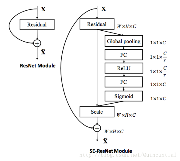
Figure 3. The schema of the original Residual module (left) and the SE-ResNet module (right).

残留网络及其变种已经证明在学习深度表示方面非常有效。我们开发了一系列的SE块，分别与ResNet[9]，ResNeXt[43]和Inception-ResNet[38]集成。图3描述了SE-ResNet模块的架构。在这里，SE块变换$\mathbf{F}_{tr}$被认为是残差模块的非恒等分支。压缩和激励都在恒等分支相加之前起作用。

图3。 最初的Residual模块架构(左)和SE-ResNet模块架构(右)。

4. Model and Computational Complexity

An SENet is constructed by stacking a set of SE blocks. In practice, it is generated by replacing each original block (i.e. residual block) with its corresponding SE counterpart (i.e. SE-residual block). We describe the architecture of SE-ResNet-50 and SE-ResNeXt-50 in Table 1.

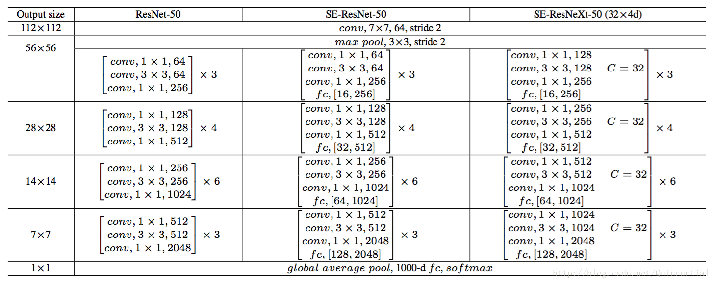
Table 1. (Left) ResNet-50. (Middle) SE-ResNet-50. (Right) SE-ResNeXt-50 with a $32\times 4d$ template. The shapes and operations with specific parameter settings of a residual building block are listed inside the brackets and the number of stacked blocks in a stage is presented outside. The inner brackets following by fc indicates the output dimension of the two fully connected layers in a SE-module.

4. 模型和计算复杂度

SENet通过堆叠一组SE块来构建。实际上，它是通过用原始块的SE对应部分（即SE残差块）替换每个原始块（即残差块）而产生的。我们在表1中描述了SE-ResNet-50和SE-ResNeXt-50的架构。

表1。(左)ResNet-50，(中)SE-ResNet-50，(右)具有$32\times 4d$模板的SE-ResNeXt-50。在括号内列出了残差构建块特定参数设置的形状和操作，并且在外部呈现了一个阶段中堆叠块的数量。fc后面的内括号表示SE模块中两个全连接层的输出维度。

For the proposed SE block to be viable in practice, it must provide an acceptable model complexity and computational overhead which is important for scalability. To illustrate the cost of the module, we take the comparison between ResNet-50 and SE-ResNet-50 as an example, where the accuracy of SE-ResNet-50 is obviously superior to ResNet-50 and approaching a deeper ResNet-101 network (shown in Table 2). ResNet-50 requires $\sim$3.86 GFLOPs in a single forward pass for a $224\times224$ pixel input image. Each SE block makes use of a global average pooling operation in the squeeze phase and two small fully connected layers in the excitation phase, followed by an inexpensive channel-wise scaling operation. In aggregate, SE-ResNet-50 requires $\sim$3.87 GFLOPs, corresponding to only a $0.26\%$ relative increase over the original ResNet-50.

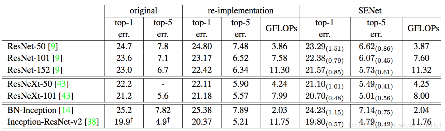
Table 2. Single-crop error rates (%) on the ImageNet validation set and complexity comparisons. The original column refers to the results reported in the original papers. To enable a fair comparison, we re-train the baseline models and report the scores in the re-implementation column. The SENet column refers the corresponding architectures in which SE blocks have been added. The numbers in brackets denote the performance improvement over the re-implemented baselines. † indicates that the model has been evaluated on the non-blacklisted subset of the validation set (this is discussed in more detail in [38]), which may slightly improve results.

在实践中提出的SE块是可行的，它必须提供可接受的模型复杂度和计算开销，这对于可伸缩性是重要的。为了说明模块的成本，作为例子我们比较了ResNet-50和SE-ResNet-50，其中SE-ResNet-50的精确度明显优于ResNet-50，接近更深的ResNet-101网络（如表2所示）。对于$224\times 224$像素的输入图像，ResNet-50单次前向传播需要$\sim$ 3.86 GFLOP。每个SE块利用压缩阶段的全局平均池化操作和激励阶段中的两个小的全连接层，接下来是廉价的通道缩放操作。总的来说，SE-ResNet-50需要$\sim$ 3.87 GFLOP，相对于原始的ResNet-50只相对增加了$0.26\%$。

表2。ImageNet验证集上的单裁剪图像错误率（％）和复杂度比较。original列是指原始论文中报告的结果。为了进行公平比较，我们重新训练了基准模型，并在re-implementation列中报告分数。SENet列是指已添加SE块后对应的架构。括号内的数字表示与重新实现的基准数据相比的性能改善。†表示该模型已经在验证集的非黑名单子集上进行了评估（在[38]中有更详细的讨论），这可能稍微改善结果。

In practice, with a training mini-batch of $256$ images, a single pass forwards and backwards through ResNet-50 takes $190$ms, compared to $209$ms for SE-ResNet-50 (both timings are performed on a server with $8$ NVIDIA Titan X GPUs). We argue that it is a reasonable overhead as global pooling and small inner-product operations are less optimised in existing GPU libraries. Moreover, due to its importance for embedded device applications, we also benchmark CPU inference time for each model: for a $224\times 224$ pixel input image, ResNet-50 takes $164$ms, compared to for SE-ResNet-$50$. The small additional computational overhead required by the SE block is justified by its contribution to model performance (discussed in detail in Sec. 6).

在实践中，训练的批数据大小为256张图像，ResNet-50的一次前向传播和反向传播花费$190$ ms，而SE-ResNet-50则花费$209$ ms（两个时间都在具有$8$个NVIDIA Titan X GPU的服务器上执行）。我们认为这是一个合理的开销，因为在现有的GPU库中，全局池化和小型内积操作的优化程度较低。此外，由于其对嵌入式设备应用的重要性，我们还对每个模型的CPU推断时间进行了基准测试：对于$224\times 224$像素的输入图像，ResNet-50花费了$164$ms，相比之下，SE-ResNet-$50$花费了$167$ms。SE块所需的小的额外计算开销对于其对模型性能的贡献来说是合理的（在第6节中详细讨论）。

Next, we consider the additional parameters introduced by the proposed block. All additional parameters are contained in the two fully connected layers of the gating mechanism, which constitute a small fraction of the total network capacity. More precisely, the number of additional parameters introduced is given by:

$$\frac{2}{r} \sum_{s=1}^S N_s \cdot {C_s}^2$$ where $r$ denotes the reduction ratio (we set $r$ to $16$ in all our experiments), $S$ refers to the number of stages (where each stage refers to the collection of blocks operating on feature maps of a common spatial dimension), $C_s$ denotes the dimension of the output channels for stage $s$ and $N_s$ refers to the repeated block number. In total, SE-ResNet-50 introduces $\sim$2.5 million additional parameters beyond the $\sim$25 million parameters required by ResNet-50, corresponding to a $\sim 10\%$ increase in the total number of parameters. The majority of these additional parameters come from the last stage of the network, where excitation is performed across the greatest channel dimensions. However, we found that the comparatively expensive final stage of SE blocks could be removed at a marginal cost in performance ( <0.1% < 0.1 % <script type="math/tex" id="MathJax-Element-139"><0.1\%</script> top-1 error on ImageNet dataset) to reduce the relative parameter increase to $\sim 4\%$, which may prove useful in cases where parameter usage is a key consideration.

接下来，我们考虑所提出的块引入的附加参数。所有附加参数都包含在门机制的两个全连接层中，构成网络总容量的一小部分。更确切地说，引入的附加参数的数量由下式给出：

$$\frac{2}{r} \sum_{s=1}^S N_s \cdot {C_s}^2$$ 其中 $r$表示减少比率（我们在所有的实验中将$r$设置为 $16$）， $S$指的是阶段数量（每个阶段是指在共同的空间维度的特征映射上运行的块的集合），$C_s$表示阶段 $s$的输出通道的维度，$N_s$表示重复的块编号。总的来说，SE-ResNet-50在ResNet-50所要求的 $\sim$2500万参数之外引入了 $\sim$250万附加参数，相对增加了 $\sim 10\%$的参数总数量。这些附加参数中的大部分来自于网络的最后阶段，其中激励在最大的通道维度上执行。然而，我们发现SE块相对昂贵的最终阶段可以在性能的边际成本（ImageNet数据集上 <0.1% < 0.1 % <script type="math/tex" id="MathJax-Element-152"><0.1 \%</script>的top-1错误率）上被移除，将相对参数增加减少到 $\sim 4\%$，这在参数使用是关键考虑的情况下可能证明是有用的。

5. Implementation

During training, we follow standard practice and perform data augmentation with random-size cropping [39] to $224\times 224$ pixels ($299\times 299$ for Inception-ResNet-v2 [38] and SE-Inception-ResNet-v2) and random horizontal flipping. Input images are normalised through mean channel subtraction. In addition, we adopt the data balancing strategy described in [32] for mini-batch sampling to compensate for the uneven distribution of classes. The networks are trained on our distributed learning system “ROCS” which is capable of handing efficient parallel training of large networks. Optimisation is performed using synchronous SGD with momentum 0.9 and a mini-batch size of 1024 (split into sub-batches of 32 images per GPU across 4 servers, each containing 8 GPUs). The initial learning rate is set to 0.6 and decreased by a factor of 10 every 30 epochs. All models are trained for 100 epochs from scratch, using the weight initialisation strategy described in [8].

5. 实现

在训练过程中，我们遵循标准的做法，使用随机大小裁剪[39]到$224\times 224$像素（$299\times 299$用于Inception-ResNet-v2[38]和SE-Inception-ResNet-v2）和随机的水平翻转进行数据增强。输入图像通过通道减去均值进行归一化。另外，我们采用[32]中描述的数据均衡策略进行小批量采样，以补偿类别的不均匀分布。网络在我们的分布式学习系统“ROCS”上进行训练，能够处理大型网络的高效并行训练。使用同步SGD进行优化，动量为0.9，小批量数据的大小为1024（在4个服务器的每个GPU上分成32张图像的子批次，每个服务器包含8个GPU）。初始学习率设为0.6，每30个迭代周期减少10倍。使用[8]中描述的权重初始化策略，所有模型都从零开始训练100个迭代周期。

6. Experiments

In this section we conduct extensive experiments on the ImageNet 2012 dataset [30] for the purposes: first, to explore the impact of the proposed SE block for the basic networks with different depths and second, to investigate its capacity of integrating with current state-of-the-art network architectures, which aim to a fair comparison between SENets and non-SENets rather than pushing the performance. Next, we present the results and details of the models for ILSVRC 2017 classification task. Furthermore, we perform experiments on the Places365-Challenge scene classification dataset [48] to investigate how well SENets are able to generalise to other datasets. Finally, we investigate the role of excitation and give some analysis based on experimental phenomena.

6. 实验

在这一部分，我们在ImageNet 2012数据集上进行了大量的实验[30]，其目的是：首先探索提出的SE块对不同深度基础网络的影响；其次，调查它与最先进的网络架构集成后的能力，旨在公平比较SENets和非SENets，而不是推动性能。接下来，我们将介绍ILSVRC 2017分类任务模型的结果和详细信息。此外，我们在Places365-Challenge场景分类数据集[48]上进行了实验，以研究SENets是否能够很好地泛化到其它数据集。最后，我们研究激励的作用，并根据实验现象给出了一些分析。

6.1. ImageNet Classification

The ImageNet 2012 dataset is comprised of 1.28 million training images and 50K validation images from 1000 classes. We train networks on the training set and report the top-1 and the top-5 errors using centre crop evaluations on the validation set, where $224\times 224$ pixels are cropped from each image whose shorter edge is first resized to 256 ($299\times 299$ from each image whose shorter edge is first resized to 352 for Inception-ResNet-v2 and SE-Inception-ResNet-v2).

6.1. ImageNet分类

ImageNet 2012数据集包含来自1000个类别的128万张训练图像和5万张验证图像。我们在训练集上训练网络，并在验证集上使用中心裁剪图像评估来报告top-1和top-5错误率，其中每张图像短边首先归一化为256，然后从每张图像中裁剪出$224\times 224$个像素，（对于Inception-ResNet-v2和SE-Inception-ResNet-v2，每幅图像的短边首先归一化到352，然后裁剪出$299\times 299$个像素）。

Network depth. We first compare the SE-ResNet against a collection of standard ResNet architectures. Each ResNet and its corresponding SE-ResNet are trained with identical optimisation schemes. The performance of the different networks on the validation set is shown in Table 2, which shows that SE blocks consistently improve performance across different depths with an extremely small increase in computational complexity.

网络深度。我们首先将SE-ResNet与一系列标准ResNet架构进行比较。每个ResNet及其相应的SE-ResNet都使用相同的优化方案进行训练。验证集上不同网络的性能如表2所示，表明SE块在不同深度上的网络上计算复杂度极小增加，始终提高性能。

Remarkably, SE-ResNet-50 achieves a single-crop top-5 validation error of $6.62\%$, exceeding ResNet-50 ($7.48\%$) by $0.86\%$ and approaching the performance achieved by the much deeper ResNet-101 network ($6.52\%$ top-5 error) with only half of the computational overhead ($3.87$ GFLOPs vs. $7.58$ GFLOPs). This pattern is repeated at greater depth, where SE-ResNet-101 ($6.07\%$ top-$5$ error) not only matches, but outperforms the deeper ResNet-152 network ($6.34\%$ top-5 error) by $0.27\%$. Fig.4 depicts the training and validation curves of SE-ResNets and ResNets, respectively. While it should be noted that the SE blocks themselves add depth, they do so in an extremely computationally efficient manner and yield good returns even at the point at which extending the depth of the base architecture achieves diminishing returns. Moreover, we see that the performance improvements are consistent through training across a range of different depths, suggesting that the improvements induced by SE blocks can be used in combination with adding more depth to the base architecture.

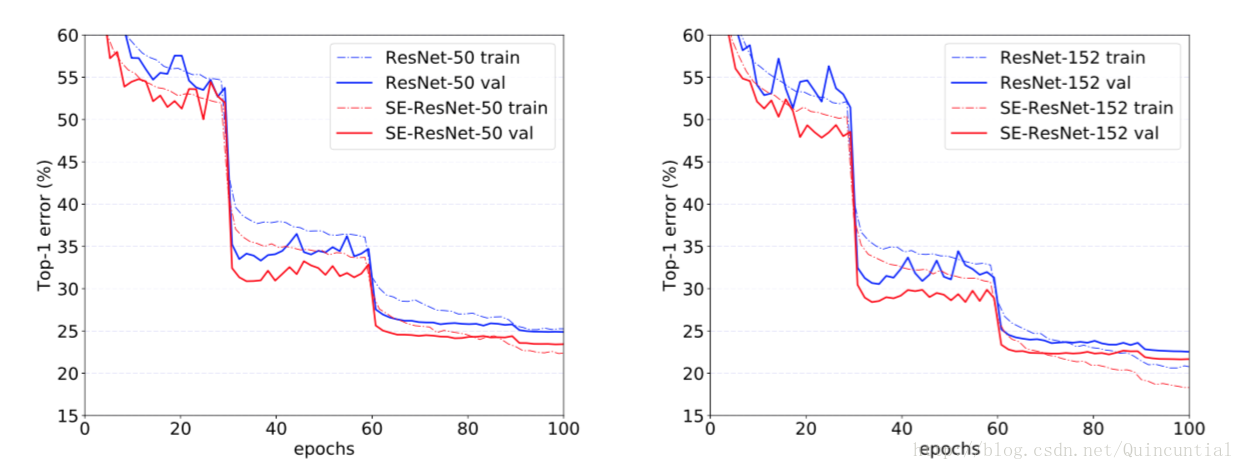
Figure 4. Training curves on ImageNet. (Left): ResNet-50 and SE-ResNet-50; (Right): ResNet-152 and SE-ResNet-152.

值得注意的是，SE-ResNet-50实现了单裁剪图像$6.62\%$的top-5验证错误率，超过了ResNet-50（$7.48\%$）$0.86\%$，接近更深的ResNet-101网络（$6.52\%$的top-5错误率），且只有ResNet-101一半的计算开销（$3.87$ GFLOPs vs. $7.58$ GFLOPs）。这种模式在更大的深度上重复，SE-ResNet-101（$6.07\%$的top-5错误率）不仅可以匹配，而且超过了更深的ResNet-152网络（$6.34\%$的top-5错误率）。图4分别描绘了SE-ResNets和ResNets的训练和验证曲线。虽然应该注意SE块本身增加了深度，但是它们的计算效率极高，即使在扩展的基础架构的深度达到收益递减的点上也能产生良好的回报。而且，我们看到通过对各种不同深度的训练，性能改进是一致的，这表明SE块引起的改进可以与增加基础架构更多深度结合使用。

图4。ImageNet上的训练曲线。(左)：ResNet-50和SE-ResNet-50；(右)：ResNet-152和SE-ResNet-152。

Integration with modern architectures. We next investigate the effect of combining SE blocks with another two state-of-the-art architectures, Inception-ResNet-v2 [38] and ResNeXt [43]. The Inception architecture constructs modules of convolutions as multibranch combinations of factorised filters, reflecting the Inception hypothesis [6] that spatial correlations and cross-channel correlations can be mapped independently. In contrast, the ResNeXt architecture asserts that richer representations can be obtained by aggregating combinations of sparsely connected (in the channel dimension) convolutional features. Both approaches introduce prior-structured correlations in modules. We construct SENet equivalents of these networks, SE-Inception-ResNet-v2 and SE-ResNeXt (the configuration of SE-ResNeXt-50 ($32\times 4d$) is given in Table 1). Like previous experiments, the same optimisation scheme is used for both the original networks and their SENet counterparts.

与现代架构集成。接下来我们将研究SE块与另外两种最先进的架构Inception-ResNet-v2[38]和ResNeXt[43]的结合效果。Inception架构将卷积模块构造为分解滤波器的多分支组合，反映了Inception假设[6]，可以独立映射空间相关性和跨通道相关性。相比之下，ResNeXt体架构断言，可以通过聚合稀疏连接（在通道维度中）卷积特征的组合来获得更丰富的表示。两种方法都在模块中引入了先前结构化的相关性。我们构造了这些网络的SENet等价物，SE-Inception-ResNet-v2和SE-ResNeXt（表1给出了SE-ResNeXt-50（$32\times 4d$）的配置）。像前面的实验一样，原始网络和它们对应的SENet网络都使用相同的优化方案。

The results given in Table 2 illustrate the significant performance improvement induced by SE blocks when introduced into both architectures. In particular, SE-ResNeXt-50 has a top-5 error of $5.49\%$ which is superior to both its direct counterpart ResNeXt-50 ($5.90\%$ top-5 error) as well as the deeper ResNeXt-101 ($5.57\%$ top-5 error), a model which has almost double the number of parameters and computational overhead. As for the experiments of Inception-ResNet-v2, we conjecture the difference of cropping strategy might lead to the gap between their reported result and our re-implemented one, as their original image size has not been clarified in [38] while we crop the $299\times 299$ region from a relative larger image (where the shorter edge is resized to 352). SE-Inception-ResNet-v2 ($4.79\%$ top-5 error) outperforms our reimplemented Inception-ResNet-v2 ($5.21\%$ top-5 error) by $0.42\%$ (a relative improvement of $8.1\%$) as well as the reported result in [38]. The optimisation curves for each network are depicted in Fig. 5, illustrating the consistency of the improvement yielded by SE blocks throughout the training process.

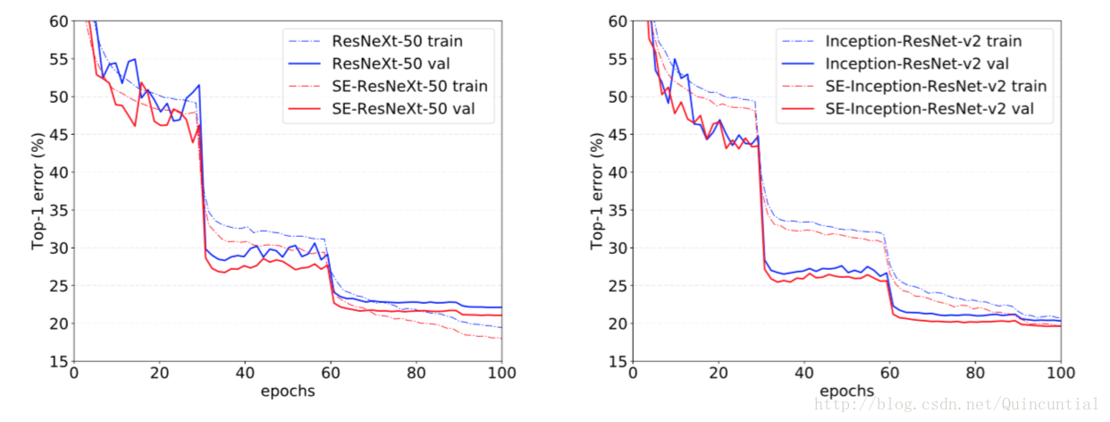
Figure 5. Training curves on ImageNet. (Left): ResNeXt-50 and SE-ResNeXt-50; (Right): Inception-ResNet-v2 and SE-Inception-ResNet-v2.

表2中给出的结果说明在将SE块引入到两种架构中会引起显著的性能改善。尤其是SE-ResNeXt-50的top-5错误率是$5.49\%$，优于于它直接对应的ResNeXt-50（$5.90\%$的top-5错误率）以及更深的ResNeXt-101（$5.57\%$的top-5错误率），这个模型几乎有两倍的参数和计算开销。对于Inception-ResNet-v2的实验，我们猜测可能是裁剪策略的差异导致了其报告结果与我们重新实现的结果之间的差距，因为它们的原始图像大小尚未在[38]中澄清，而我们从相对较大的图像（其中较短边被归一化为352）中裁剪出$299\times 299$大小的区域。SE-Inception-ResNet-v2（$4.79\%$的top-5错误率）比我们重新实现的Inception-ResNet-v2（$5.21\%$的top-5错误率）要低$0.42\%$（相对改进了$8.1\%$）也优于[38]中报告的结果。每个网络的优化曲线如图5所示，说明了在整个训练过程中SE块产生了一致的改进。

图5。ImageNet的训练曲线。(左): ResNeXt-50和SE-ResNeXt-50；(右)：Inception-ResNet-v2和SE-Inception-ResNet-v2。

Finally, we assess the effect of SE blocks when operating on a non-residual network by conducting experiments with the BN-Inception architecture [14] which provides good performance at a lower model complexity. The results of the comparison are shown in Table 2 and the training curves are shown in Fig. 6, exhibiting the same phenomena that emerged in the residual architectures. In particular, SE-BN-Inception achieves a lower top-5 error of $7.14\%$ in comparison to BN-Inception whose error rate is $7.89\%$. These experiments demonstrate that improvements induced by SE blocks can be used in combination with a wide range of architectures. Moreover, this result holds for both residual and non-residual foundations.

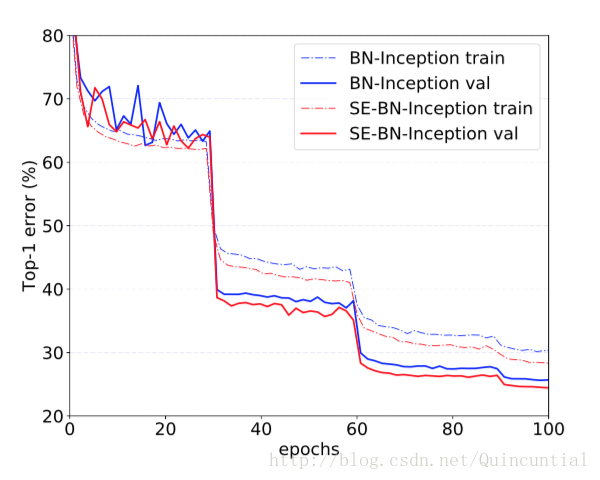
Figure 6. Training curves of BN-Inception and SE-BN-Inception on ImageNet.

最后，我们通过对BN-Inception架构[14]进行实验来评估SE块在非残差网络上的效果，该架构在较低的模型复杂度下提供了良好的性能。比较结果如表2所示，训练曲线如图6所示，表现出的现象与残差架构中出现的现象一样。尤其是与BN-Inception $7.89\%$的错误率相比，SE-BN-Inception获得了更低$7.14\%$的top-5错误。这些实验表明SE块引起的改进可以与多种架构结合使用。而且，这个结果适用于残差和非残差基础。

图6。BN-Inception和SE-BN-Inception在ImageNet上的训练曲线。

Results on ILSVRC 2017 Classification Competition. ILSVRC [30] is an annual computer vision competition which has proved to be a fertile ground for model developments in image classification. The training and validation data of the ILSVRC 2017 classification task are drawn from the ImageNet 2012 dataset, while the test set consists of an additional unlabelled 100K images. For the purposes of the competition, the top-5 error metric is used to rank entries.

**ILSVRC 2017分类竞赛的结果。**ILSVRC[30]是一个年度计算机视觉竞赛，被证明是图像分类模型发展的沃土。ILSVRC 2017分类任务的训练和验证数据来自ImageNet 2012数据集，而测试集包含额外的未标记的10万张图像。为了竞争的目的，使用top-5错误率度量来对输入条目进行排序。

SENets formed the foundation of our submission to the challenge where we won first place. Our winning entry comprised a small ensemble of SENets that employed a standard multi-scale and multi-crop fusion strategy to obtain a $2.251\%$ top-5 error on the test set. This result represents a $\sim 25\%$ relative improvement on the winning entry of 2016 ($2.99\%$ top-5 error). One of our high-performing networks is constructed by integrating SE blocks with a modified ResNeXt [43] (details of the modifications are provided in Appendix A). We compare the proposed architecture with the state-of-the-art models on the ImageNet validation set in Table 3. Our model achieves a top-1 error of $18.68\%$ and a top-5 error of $4.47\%$ using a $224\times 224$ centre crop evaluation on each image (where the shorter edge is first resized to 256). To enable a fair comparison with previous models, we also provide a $320\times 320$ centre crop evaluation, obtaining the lowest error rate under both the top-1 ($17.28\%$) and the top-5 ($3.79\%$) error metrics.

Table 3. Single-crop error rates of state-of-the-art CNNs on ImageNet validation set. The size of test crop is $224\times 224$ and $320\times 320$/$299\times299$ as in [10]. Our proposed model, SENet, shows a significant performance improvement on prior work.

SENets是我们在挑战中赢得第一名的基础。我们的获胜输入由一小群SENets组成，它们采用标准的多尺度和多裁剪图像融合策略，在测试集上获得了$2.251\%$的top-5错误率。这个结果表示在2016年获胜输入（$2.99\%$的top-5错误率）的基础上相对改进了$\sim 25\%$。我们的高性能网络之一是将SE块与修改后的ResNeXt[43]集成在一起构建的（附录A提供了这些修改的细节）。在表3中我们将提出的架构与最新的模型在ImageNet验证集上进行了比较。我们的模型在每一张图像使用$224\times 224$中间裁剪评估（短边首先归一化到256）取得了$18.68\%$的top-1错误率和$4.47\%$的top-5错误率。为了与以前的模型进行公平的比较，我们也提供了$320\times 320$的中心裁剪图像评估，在top-1($17.28\%$)和top-5($3.79\%$)的错误率度量中获得了最低的错误率。

表3。最新的CNNs在ImageNet验证集上单裁剪图像的错误率。测试的裁剪图像大小是$224\times 224$和[10]中的$320\times 320$/$299\times299$。与前面的工作相比，我们提出的模型SENet表现出了显著的改进。

6.2. Scene Classification

Large portions of the ImageNet dataset consist of images dominated by single objects. To evaluate our proposed model in more diverse scenarios, we also evaluate it on the Places365-Challenge dataset [48] for scene classification. This dataset comprises 8 million training images and 36, 500 validation images across 365 categories. Relative to classification, the task of scene understanding can provide a better assessment of the ability of a model to generalise well and handle abstraction, since it requires the capture of more complex data associations and robustness to a greater level of appearance variation.

6.2. 场景分类

ImageNet数据集的大部分由单个对象支配的图像组成。为了在更多不同的场景下评估我们提出的模型，我们还在Places365-Challenge数据集[48]上对场景分类进行评估。该数据集包含800万张训练图像和365个类别的36500张验证图像。相对于分类，场景理解的任务可以更好地评估模型泛化和处理抽象的能力，因为它需要捕获更复杂的数据关联以及对更大程度外观变化的鲁棒性。

We use ResNet-152 as a strong baseline to assess the effectiveness of SE blocks and follow the evaluation protocol in [33]. Table 4 shows the results of training a ResNet-152 model and a SE-ResNet-152 for the given task. Specifically, SE-ResNet-152 ($11.01\%$ top-5 error) achieves a lower validation error than ResNet-152 ($11.61\%$ top-5 error), providing evidence that SE blocks can perform well on different datasets. This SENet surpasses the previous state-of-the-art model Places-365-CNN [33] which has a top-5 error of $11.48\%$ on this task.

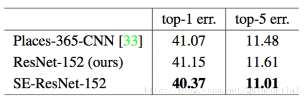
Table 4. Single-crop error rates (%) on the Places365 validation set.

我们使用ResNet-152作为强大的基线来评估SE块的有效性，并遵循[33]中的评估协议。表4显示了针对给定任务训练ResNet-152模型和SE-ResNet-152的结果。具体而言，SE-ResNet-152（$11.01\%$的top-5错误率）取得了比ResNet-152（$11.61\%$的top-5错误率）更低的验证错误率，证明了SE块可以在不同的数据集上表现良好。这个SENet超过了先前的最先进的模型Places-365-CNN [33]，它在这个任务上有$11.48\%$的top-5错误率。

表4。Places365验证集上的单裁剪图像错误率(%)。

6.3. Analysis and Discussion

Reduction ratio. The reduction ratio $r$ introduced in Eqn. (5) is an important hyperparameter which allows us to vary the capacity and computational cost of the SE blocks in the model. To investigate this relationship, we conduct experiments based on the SE-ResNet-50 architecture for a range of different $r$ values. The comparison in Table 5 reveals that performance does not improve monotonically with increased capacity. This is likely to be a result of enabling the SE block to overfit the channel interdependencies of the training set. In particular, we found that setting $r=16$ achieved a good tradeoff between accuracy and complexity and consequently, we used this value for all experiments.

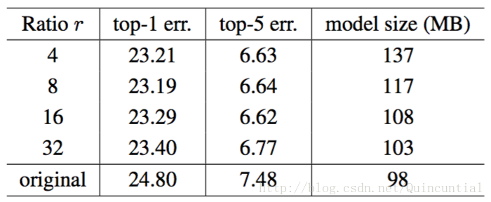
Table 5. Single-crop error rates (%) on the ImageNet validation set and corresponding model sizes for the SE-ResNet-50 architecture at different reduction ratios $r$. Here original refers to ResNet-50.

6.3. 分析和讨论

减少比率。公式（5）中引入的减少比率$r$是一个重要的超参数，它允许我们改变模型中SE块的容量和计算成本。为了研究这种关系，我们基于SE-ResNet-50架构进行了一系列不同$r$值的实验。表5中的比较表明，性能并没有随着容量的增加而单调上升。这可能是使SE块能够过度拟合训练集通道依赖性的结果。尤其是我们发现设置$r=16$在精度和复杂度之间取得了很好的平衡，因此我们将这个值用于所有的实验。

表5。 ImageNet验证集上单裁剪图像的错误率(%)和SE-ResNet-50架构在不同减少比率$r$下的模型大小。这里original指的是ResNet-50。

The role of Excitation. While SE blocks have been empirically shown to improve network performance, we would also like to understand how the self-gating excitation mechanism operates in practice. To provide a clearer picture of the behaviour of SE blocks, in this section we study example activations from the SE-ResNet-50 model and examine their distribution with respect to different classes at different blocks. Specifically, we sample four classes from the ImageNet dataset that exhibit semantic and appearance diversity, namely goldfish, pug, plane and cliff (example images from these classes are shown in Fig. 7). We then draw fifty samples for each class from the validation set and compute the average activations for fifty uniformly sampled channels in the last SE block in each stage (immediately prior to downsampling) and plot their distribution in Fig. 8. For reference, we also plot the distribution of average activations across all 1000 classes.

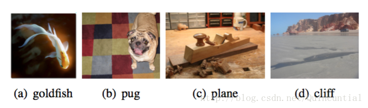
Figure 7. Example images from the four classes of ImageNet.

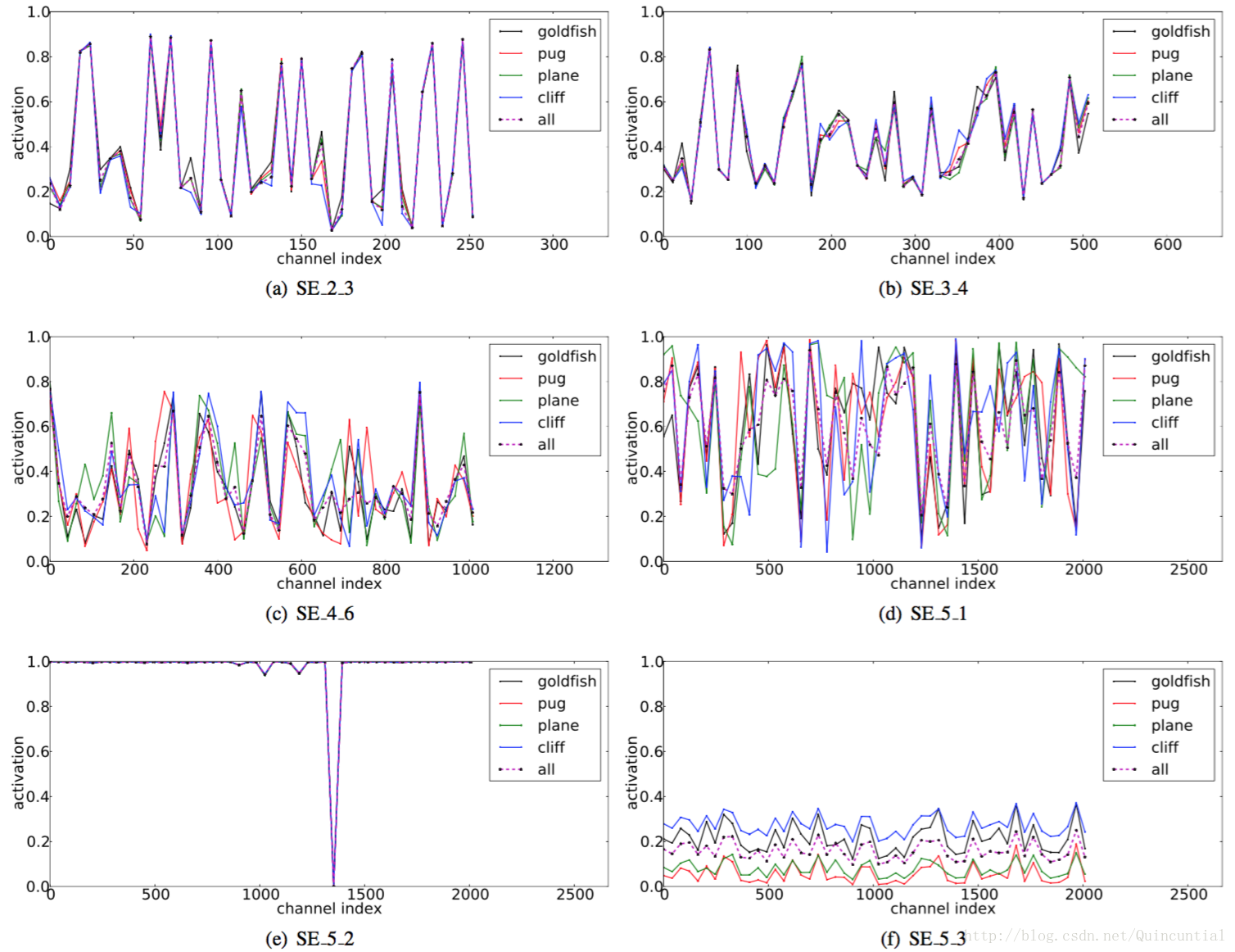
Figure 8. Activations induced by Excitation in the different modules of SE-ResNet-50 on ImageNet. The module is named as “SE stageID blockID”.

激励的作用。虽然SE块从经验上显示出其可以改善网络性能，但我们也想了解自门激励机制在实践中是如何运作的。为了更清楚地描述SE块的行为，本节我们研究SE-ResNet-50模型的样本激活，并考察它们在不同块不同类别下的分布情况。具体而言，我们从ImageNet数据集中抽取了四个类，这些类表现出语义和外观多样性，即金鱼，哈巴狗，刨和悬崖（图7中显示了这些类别的示例图像）。然后，我们从验证集中为每个类抽取50个样本，并计算每个阶段最后的SE块中50个均匀采样通道的平均激活（紧接在下采样之前），并在图8中绘制它们的分布。作为参考，我们也绘制所有1000个类的平均激活分布。

图7。ImageNet中四个类别的示例图像。

图8。SE-ResNet-50不同模块在ImageNet上由Excitation引起的激活。模块名为“SE stageID blockID”。

We make the following three observations about the role of Excitation in SENets. First, the distribution across different classes is nearly identical in lower layers, e.g. SE_2_3. This suggests that the importance of feature channels is likely to be shared by different classes in the early stages of the network. Interestingly however, the second observation is that at greater depth, the value of each channel becomes much more class-specific as different classes exhibit different preferences to the discriminative value of features e.g. SE_4_6 and SE_5_1. The two observations are consistent with findings in previous work [21, 46], namely that lower layer features are typically more general (i.e. class agnostic in the context of classification) while higher layer features have greater specificity. As a result, representation learning benefits from the recalibration induced by SE blocks which adaptively facilitates feature extraction and specialisation to the extent that it is needed. Finally, we observe a somewhat different phenomena in the last stage of the network. SE_5_2 exhibits an interesting tendency towards a saturated state in which most of the activations are close to 1 and the remainder are close to 0. At the point at which all activations take the value 1, this block would become a standard residual block. At the end of the network in the SE_5_3 (which is immediately followed by global pooling prior before classifiers), a similar pattern emerges over different classes, up to a slight change in scale (which could be tuned by the classifiers). This suggests that SE_5_2 and SE_5_3 are less important than previous blocks in providing recalibration to the network. This finding is consistent with the result of the empirical investigation in Sec. 4 which demonstrated that the overall parameter count could be significantly reduced by removing the SE blocks for the last stage with only a marginal loss of performance (< $0.1\%$ top-1 error).

我们对SENets中Excitation的作用提出以下三点看法。首先，不同类别的分布在较低层中几乎相同，例如，SE_2_3。这表明在网络的最初阶段特征通道的重要性很可能由不同的类别共享。然而有趣的是，第二个观察结果是在更大的深度，每个通道的值变得更具类别特定性，因为不同类别对特征的判别性值具有不同的偏好。SE_4_6和SE_5_1。这两个观察结果与以前的研究结果一致[21,46]，即低层特征通常更普遍（即分类中不可知的类别），而高层特征具有更高的特异性。因此，表示学习从SE块引起的重新校准中受益，其自适应地促进特征提取和专业化到所需要的程度。最后，我们在网络的最后阶段观察到一个有些不同的现象。SE_5_2呈现出朝向饱和状态的有趣趋势，其中大部分激活接近于1，其余激活接近于0。在所有激活值取1的点处，该块将成为标准残差块。在网络的末端SE_5_3中（在分类器之前紧接着是全局池化），类似的模式出现在不同的类别上，尺度上只有轻微的变化（可以通过分类器来调整）。这表明，SE_5_2和SE_5_3在为网络提供重新校准方面比前面的块更不重要。这一发现与第四节实证研究的结果是一致的，这表明，通过删除最后一个阶段的SE块，总体参数数量可以显著减少，性能只有一点损失（<$0.1\%$的top-1错误率）。

7. Conclusion

In this paper we proposed the SE block, a novel architectural unit designed to improve the representational capacity of a network by enabling it to perform dynamic channel-wise feature recalibration. Extensive experiments demonstrate the effectiveness of SENets which achieve state-of-the-art performance on multiple datasets. In addition, they provide some insight into the limitations of previous architectures in modelling channel-wise feature dependencies, which we hope may prove useful for other tasks requiring strong discriminative features. Finally, the feature importance induced by SE blocks may be helpful to related fields such as network pruning for compression.

7. 结论

在本文中，我们提出了SE块，这是一种新颖的架构单元，旨在通过使网络能够执行动态通道特征重新校准来提高网络的表示能力。大量实验证明了SENets的有效性，其在多个数据集上取得了最先进的性能。此外，它们还提供了一些关于以前架构在建模通道特征依赖性上的局限性的洞察，我们希望可能证明SENets对其它需要强判别性特征的任务是有用的。最后，由SE块引起的特征重要性可能有助于相关领域，例如为了压缩的网络修剪。

Acknowledgements. We would like to thank Professor Andrew Zisserman for his helpful comments and Samuel Albanie for his discussions and writing edit for the paper. We would like to thank Chao Li for his contributions in the memory optimisation of the training system. Li Shen is supported by the Office of the Director of National Intelligence (ODNI), Intelligence Advanced Research Projects Activity (IARPA), via contract number 2014-14071600010. The views and conclusions contained herein are those of the author and should not be interpreted as necessarily representing the official policies or endorsements, either expressed or implied, of ODNI, IARPA, or the U.S. Government. The U.S. Government is authorized to reproduce and distribute reprints for Governmental purpose notwithstanding any copyright annotation thereon.

致谢。我们要感谢Andrew Zisserman教授的有益评论，并感谢Samuel Albanie的讨论并校订论文。我们要感谢Chao Li在训练系统内存优化方面的贡献。Li Shen由国家情报总监(ODNI)，先期研究计划中心（IARPA）资助，合同号为2014-14071600010。本文包含的观点和结论属于作者的观点和结论，不应理解为ODNI，IARPA或美国政府明示或暗示的官方政策或认可。尽管有任何版权注释，美国政府有权为政府目的复制和分发重印。

References

[1] S. Bell, C. L. Zitnick, K. Bala, and R. Girshick. Inside-outside net: Detecting objects in context with skip pooling and recurrent neural networks. In CVPR, 2016.

[2] T. Bluche. Joint line segmentation and transcription for end-to-end handwritten paragraph recognition. In NIPS, 2016.

[3] C.Cao, X.Liu, Y.Yang, Y.Yu, J.Wang, Z.Wang, Y.Huang, L. Wang, C. Huang, W. Xu, D. Ramanan, and T. S. Huang. Look and think twice: Capturing top-down visual attention with feedback convolutional neural networks. In ICCV, 2015.

[4] L. Chen, H. Zhang, J. Xiao, L. Nie, J. Shao, W. Liu, and T. Chua. SCA-CNN: Spatial and channel-wise attention in convolutional networks for image captioning. In CVPR, 2017.

[5] Y. Chen, J. Li, H. Xiao, X. Jin, S. Yan, and J. Feng. Dual path networks. arXiv:1707.01629, 2017.

[6] F. Chollet. Xception: Deep learning with depthwise separable convolutions. In CVPR, 2017.

[7] J. S. Chung, A. Senior, O. Vinyals, and A. Zisserman. Lip reading sentences in the wild. In CVPR, 2017.

[8] K. He, X. Zhang, S. Ren, and J. Sun. Delving deep into rectifiers: Surpassing human-level performance on ImageNet classification. In ICCV, 2015.

[9] K. He, X. Zhang, S. Ren, and J. Sun. Deep residual learning for image recognition. In CVPR, 2016.

[10] K. He, X. Zhang, S. Ren, and J. Sun. Identity mappings in deep residual networks. In ECCV, 2016.

[11] S. Hochreiter and J. Schmidhuber. Long short-term memory. Neural computation, 1997.

[12] G. Huang, Z. Liu, K. Q. Weinberger, and L. Maaten. Densely connected convolutional networks. In CVPR, 2017.

[13] Y. Ioannou, D. Robertson, R. Cipolla, and A. Criminisi. Deep roots: Improving CNN efficiency with hierarchical filter groups. In CVPR, 2017.

[14] S. Ioffe and C. Szegedy. Batch normalization: Accelerating deep network training by reducing internal covariate shift. In ICML, 2015.

[15] L. Itti and C. Koch. Computational modelling of visual attention. Nature reviews neuroscience, 2001.

[16] L. Itti, C. Koch, and E. Niebur. A model of saliency-based visual attention for rapid scene analysis. IEEE TPAMI, 1998.

[17] M. Jaderberg, K. Simonyan, A. Zisserman, and K. Kavukcuoglu. Spatial transformer networks. In NIPS, 2015.

[18] M. Jaderberg, A. Vedaldi, and A. Zisserman. Speeding up convolutional neural networks with low rank expansions. In BMVC, 2014.

[19] A. Krizhevsky, I. Sutskever, and G. E. Hinton. ImageNet classification with deep convolutional neural networks. In NIPS, 2012.

[20] H. Larochelle and G. E. Hinton. Learning to combine foveal glimpses with a third-order boltzmann machine. In NIPS, 2010.

[21] H. Lee, R. Grosse, R. Ranganath, and A. Y. Ng. Convolutional deep belief networks for scalable unsupervised learning of hierarchical representations. In ICML, 2009.

[22] M. Lin, Q. Chen, and S. Yan. Network in network. arXiv:1312.4400, 2013.

[23] J. Long, E. Shelhamer, and T. Darrell. Fully convolutional networks for semantic segmentation. In CVPR, 2015.

[24] A. Miech, I. Laptev, and J. Sivic. Learnable pooling with context gating for video classification. arXiv:1706.06905, 2017.

[25] V. Mnih, N. Heess, A. Graves, and K. Kavukcuoglu. Recurrent models of visual attention. In NIPS, 2014.

[26] V. Nair and G. E. Hinton. Rectified linear units improve restricted boltzmann machines. In ICML, 2010.

[27] A. Newell, K. Yang, and J. Deng. Stacked hourglass networks for human pose estimation. In ECCV, 2016.

[28] B. A. Olshausen, C. H. Anderson, and D. C. V. Essen. A neurobiological model of visual attention and invariant pattern recognition based on dynamic routing of information. Journal of Neuroscience, 1993.

[29] S. Ren, K. He, R. Girshick, and J. Sun. Faster R-CNN: Towards real-time object detection with region proposal networks. In NIPS, 2015.

[30] O. Russakovsky, J. Deng, H. Su, J. Krause, S. Satheesh, S. Ma, Z. Huang, A. Karpathy, A. Khosla, M. Bernstein, A. C. Berg, and L. Fei-Fei. ImageNet large scale visual recognition challenge. IJCV, 2015.

[31] J. Sanchez, F. Perronnin, T. Mensink, and J. Verbeek. Image classification with the fisher vector: Theory and practice. RR-8209, INRIA, 2013.

[32] L. Shen, Z. Lin, and Q. Huang. Relay backpropagation for effective learning of deep convolutional neural networks. In ECCV, 2016.

[33] L. Shen, Z. Lin, G. Sun, and J. Hu. Places401 and places365 models. https://github.com/lishen-shirley/ Places2-CNNs, 2016.

[34] L. Shen, G. Sun, Q. Huang, S. Wang, Z. Lin, and E. Wu. Multi-level discriminative dictionary learning with application to large scale image classification. IEEE TIP, 2015.

[35] K. Simonyan and A. Zisserman. Very deep convolutional networks for large-scale image recognition. In ICLR, 2015.

[36] R. K. Srivastava, K. Greff, and J. Schmidhuber. Training very deep networks. In NIPS, 2015.

[37] M. F. Stollenga, J. Masci, F. Gomez, and J. Schmidhuber. Deep networks with internal selective attention through feedback connections. In NIPS, 2014.

[38] C.Szegedy, S.Ioffe, V.Vanhoucke, and A.Alemi. Inception-v4, inception-resnet and the impact of residual connections on learning. arXiv:1602.07261, 2016.

[39] C. Szegedy, W. Liu, Y. Jia, P. Sermanet, S. Reed, D. Anguelov, D. Erhan, V. Vanhoucke, and A. Rabinovich. Going deeper with convolutions. In CVPR, 2015.

[40] C.Szegedy, V.Vanhoucke, S.Ioffe, J.Shlens, and Z.Wojna. Rethinking the inception architecture for computer vision. In CVPR, 2016.

[41] A. Toshev and C. Szegedy. DeepPose: Human pose estimation via deep neural networks. In CVPR, 2014.

[42] F. Wang, M. Jiang, C. Qian, S. Yang, C. Li, H. Zhang, X. Wang, and X. Tang. Residual attention network for image classification. In CVPR, 2017.

[43] S. Xie, R. Girshick, P. Dollar, Z. Tu, and K. He. Aggregated residual transformations for deep neural networks. In CVPR, 2017.

[44] K. Xu, J. Ba, R. Kiros, K. Cho, A. Courville, R. Salakhudinov, R. Zemel, and Y. Bengio. Show, attend and tell: Neural image caption generation with visual attention. In ICML, 2015.

[45] J. Yang, K. Yu, Y. Gong, and T. Huang. Linear spatial pyramid matching using sparse coding for image classification. In CVPR, 2009.

[46] J. Yosinski, J. Clune, Y. Bengio, and H. Lipson. How transferable are features in deep neural networks? In NIPS, 2014.

[47] X. Zhang, Z. Li, C. C. Loy, and D. Lin. Polynet: A pursuit of structural diversity in very deep networks. In CVPR, 2017.

[48] B. Zhou, A. Lapedriza, A. Khosla, A. Oliva, and A. Torralba. Places: A 10 million image database for scene recognition. IEEE TPAMI, 2017.

A. ILSVRC 2017 Classification Competition Entry Details

The SENet in Table 3 is constructed by integrating SE blocks to a modified version of the $64\times 4d$ ResNeXt-152 that extends the original ResNeXt-101 [43] by following the block stacking of ResNet-152 [9]. More differences to the design and training (beyond the use of SE blocks) were as follows: (a) The number of first $1\times 1$ convolutional channels for each bottleneck building block was halved to reduce the computation cost of the network with a minimal decrease in performance. (b) The first $7\times 7$ convolutional layer was replaced with three consecutive $3\times 3$ convolutional layers. (c) The down-sampling projection $1\times 1$ with stride-2 convolution was replaced with a $3\times 3$ stride-2 convolution to preserve information. (d) A dropout layer (with a drop ratio of 0.2) was inserted before the classifier layer to prevent overfitting. (e) Label-smoothing regularisation (as introduced in [40]) was used during training. (f) The parameters of all BN layers were frozen for the last few training epochs to ensure consistency between training and testing. (g) Training was performed with 8 servers (64 GPUs) in parallelism to enable a large batch size (2048) and initial learning rate of 1.0.

A. ILSVRC 2017分类竞赛输入细节

表3中的SENet是通过将SE块集成到$64\times 4d$的ResNeXt-152的修改版本中构建的，通过遵循ResNet-152[9]的块堆叠来扩展原始ResNeXt-101[43]。更多设计和训练差异（除了SE块的使用之外）如下：（a）对于每个瓶颈构建块，首先$1\times 1$卷积通道的数量减半，以性能下降最小的方式降低网络的计算成本。（b）第一个$7\times 7$卷积层被三个连续的$3\times 3$卷积层所取代。（c）步长为2的$1\times 1$卷积的下采样投影被替换步长为2的$3\times 3$卷积以保留信息。（d）在分类器层之前插入一个丢弃层（丢弃比为0.2）以防止过拟合。（e）训练期间使用标签平滑正则化（如[40]中所介绍的）。（f）在最后几个训练迭代周期，所有BN层的参数都被冻结，以确保训练和测试之间的一致性。（g）使用8个服务器（64个GPU）并行执行培训，以实现大批量数据大小（2048），初始学习率为1.0。