Conv Nets: A Modular Perspective

Conv Nets: A Modular Perspective

Posted on July 8, 2014

neural networks, deep learning, convolutional neural networks, modular neural networks

Introduction

In the last few years, deep neural networks have lead to breakthrough results on a variety of pattern recognition problems, such as computer vision and voice recognition. One of the essential components leading to these results has been a special kind of neural network called aconvolutional neural network.

At its most basic, convolutional neural networks can be thought of as a kind of neural network that uses many identical copies of the same neuron.1 This allows the network to have lots of neurons and express computationally large models while keeping the number of actual parameters – the values describing how neurons behave – that need to be learned fairly small.

A 2D Convolutional Neural Network

This trick of having multiple copies of the same neuron is roughly analogous to the abstraction of functions in mathematics and computer science. When programming, we write a function once and use it in many places – not writing the same code a hundred times in different places makes it faster to program, and results in fewer bugs. Similarly, a convolutional neural network can learn a neuron once and use it in many places, making it easier to learn the model and reducing error.

Structure of Convolutional Neural Networks

Suppose you want a neural network to look at audio samples and predict whether a human is speaking or not. Maybe you want to do more analysis if someone is speaking.

You get audio samples at different points in time. The samples are evenly spaced.

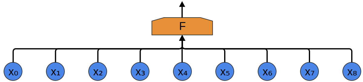
The simplest way to try and classify them with a neural network is to just connect them all to a fully-connected layer. There are a bunch of different neurons, and every input connects to every neuron.

A more sophisticated approach notices a kind of symmetry in the properties it’s useful to look for in the data. We care a lot about local properties of the data: What frequency of sounds are there around a given time? Are they increasing or decreasing? And so on.

We care about the same properties at all points in time. It’s useful to know the frequencies at the beginning, it’s useful to know the frequencies in the middle, and it’s also useful to know the frequencies at the end. Again, note that these are local properties, in that we only need to look at a small window of the audio sample in order to determine them.

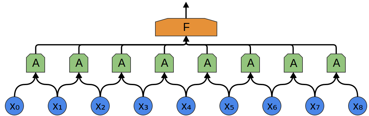
So, we can create a group of neurons,  A A, that look at small time segments of our data.2  A A looks at all such segments, computing certain features. Then, the output of this convolutional layer is fed into a fully-connected layer,  F F.

In the above example,  A A only looked at segments consisting of two points. This isn’t realistic. Usually, a convolution layer’s window would be much larger.

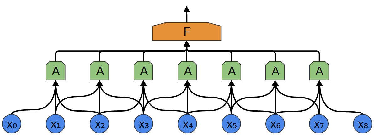
In the following example,  A A looks at 3 points. That isn’t realistic either – sadly, it’s tricky to visualize  A A connecting to lots of points.

One very nice property of convolutional layers is that they’re composable. You can feed the output of one convolutional layer into another. With each layer, the network can detect higher-level, more abstract features.

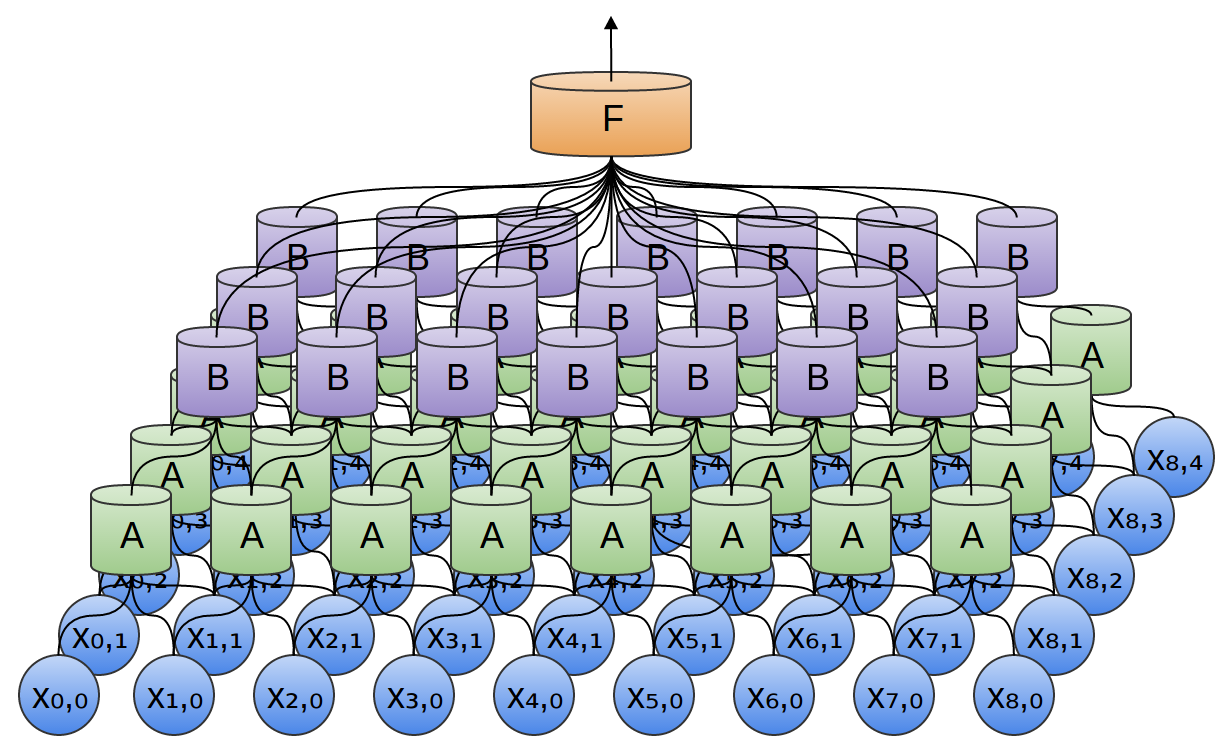
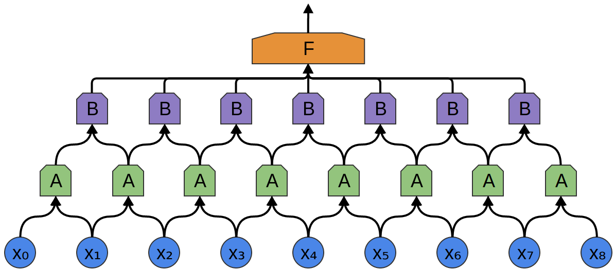
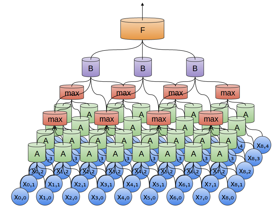
In the following example, we have a new group of neurons,  B B.  B B is used to create another convolutional layer stacked on top of the previous one.

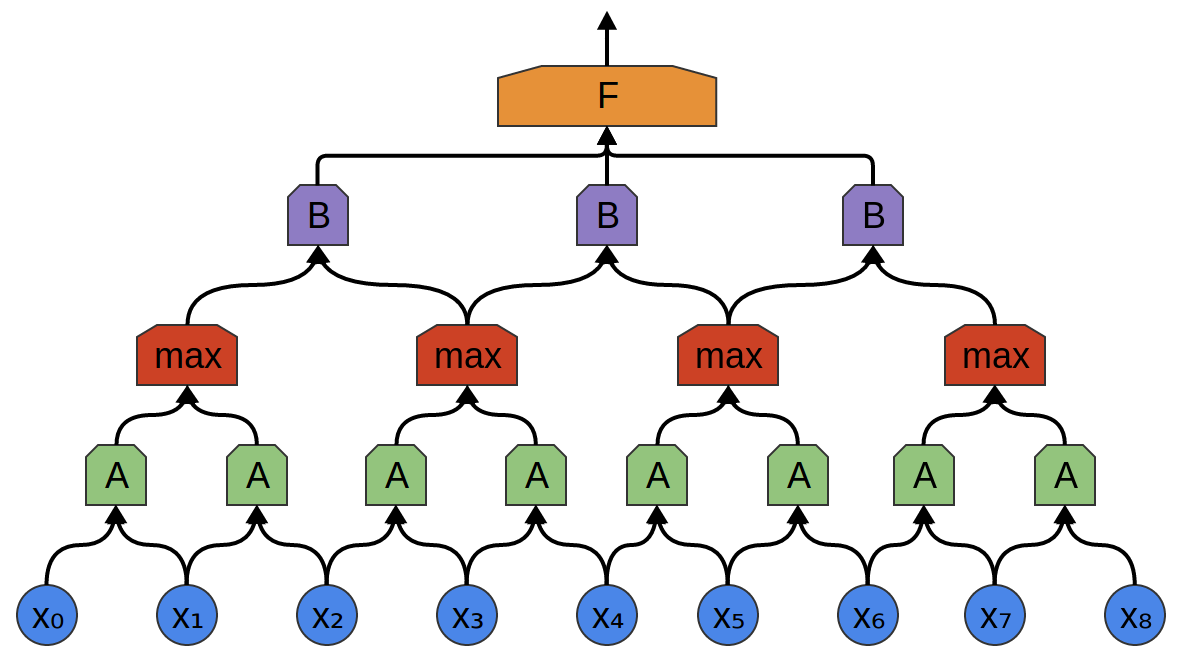
Convolutional layers are often interweaved with pooling layers. In particular, there is a kind of layer called a max-pooling layer that is extremely popular.

Often, from a high level perspective, we don’t care about the precise point in time a feature is present. If a shift in frequency occurs slightly earlier or later, does it matter?

A max-pooling layer takes the maximum of features over small blocks of a previous layer. The output tells us if a feature was present in a region of the previous layer, but not precisely where.

Max-pooling layers kind of “zoom out”. They allow later convolutional layers to work on larger sections of the data, because a small patch after the pooling layer corresponds to a much larger patch before it. They also make us invariant to some very small transformations of the data.

In our previous examples, we’ve used 1-dimensional convolutional layers. However, convolutional layers can work on higher-dimensional data as well. In fact, the most famous successes of convolutional neural networks are applying 2D convolutional neural networks to recognizing images.

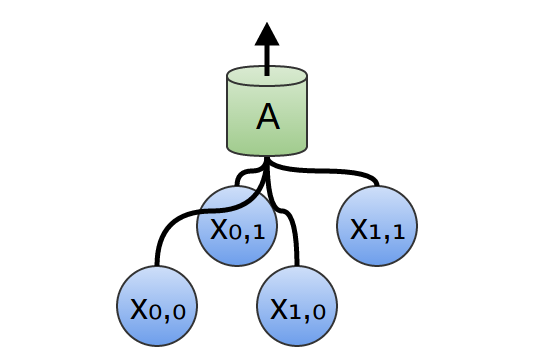
In a 2-dimensional convolutional layer, instead of looking at segments,  A A will now look at patches.

For each patch,  A A will compute features. For example, it might learn to detect the presence of an edge. Or it might learn to detect a texture. Or perhaps a contrast between two colors.

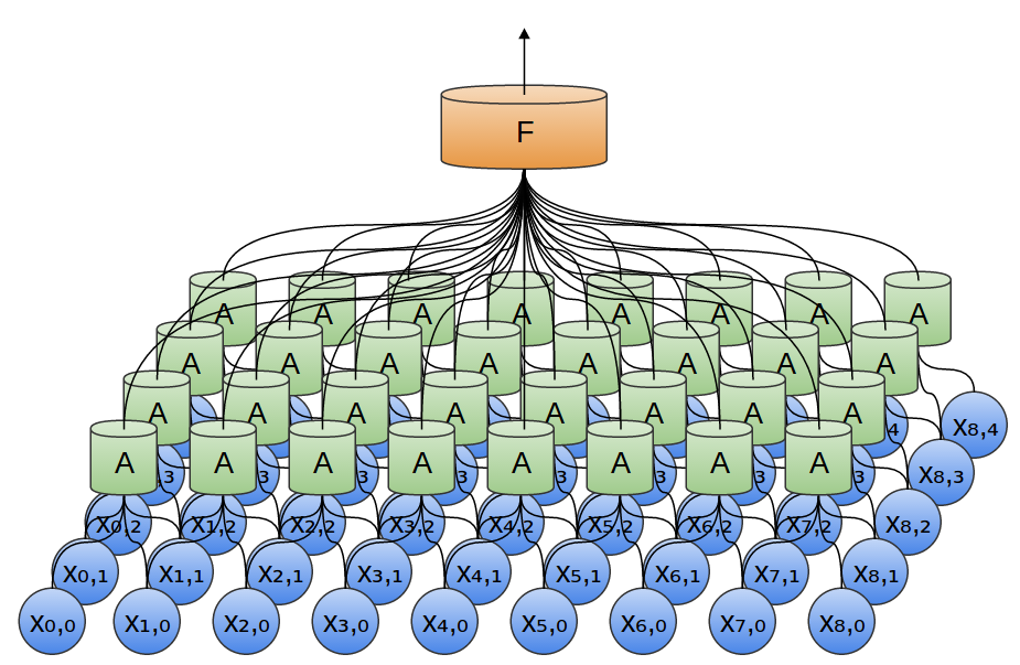
In the previous example, we fed the output of our convolutional layer into a fully-connected layer. But we can also compose two convolutional layers, as we did in the one dimensional case.

We can also do max pooling in two dimensions. Here, we take the maximum of features over a small patch.

What this really boils down to is that, when considering an entire image, we don’t care about the exact position of an edge, down to a pixel. It’s enough to know where it is to within a few pixels.

Three-dimensional convolutional networks are also sometimes used, for data like videos or volumetric data (eg. 3D medical scans). However, they are not very widely used, and much harder to visualize.

Now, we previously said that  A A was a group of neurons. We should be a bit more precise about this: what is  A A exactly?

In traditional convolutional layers,  A A is a bunch of neurons in parallel, that all get the same inputs and compute different features.

For example, in a 2-dimensional convolutional layer, one neuron might detect horizontal edges, another might detect vertical edges, and another might detect green-red color contrasts.

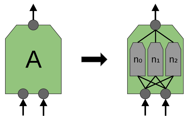
That said, in the recent paper ‘Network in Network’ (Lin et al. (2013)), a new “Mlpconv” layer is proposed. In this model,  A A would have multiple layers of neurons, with the final layer outputting higher level features for the region. In the paper, the model achieves some very impressive results, setting new state of the art on a number of benchmark datasets.

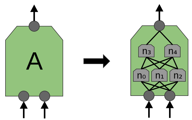
That said, for the purposes of this post, we will focus on standard convolutional layers. There’s already enough for us to consider there!

Results of Convolutional Neural Networks

Earlier, we alluded to recent breakthroughs in computer vision using convolutional neural networks. Before we go on, I’d like to briefly discuss some of these results as motivation.

In 2012, Alex Krizhevsky, Ilya Sutskever, and Geoff Hinton blew existing image classification results out of the water (Krizehvsky et al. (2012)).

Their progress was the result of combining together a bunch of different pieces. They used GPUs to train a very large, deep, neural network. They used a new kind of neuron (ReLUs) and a new technique to reduce a problem called ‘overfitting’ (DropOut). They used a very large dataset with lots of image categories (ImageNet). And, of course, it was a convolutional neural network.

Their architecture, illustrated below, was very deep. It has 5 convolutional layers,3 with pooling interspersed, and three fully-connected layers. The early layers are split over the two GPUs.

From  Krizehvsky et al. (2012)

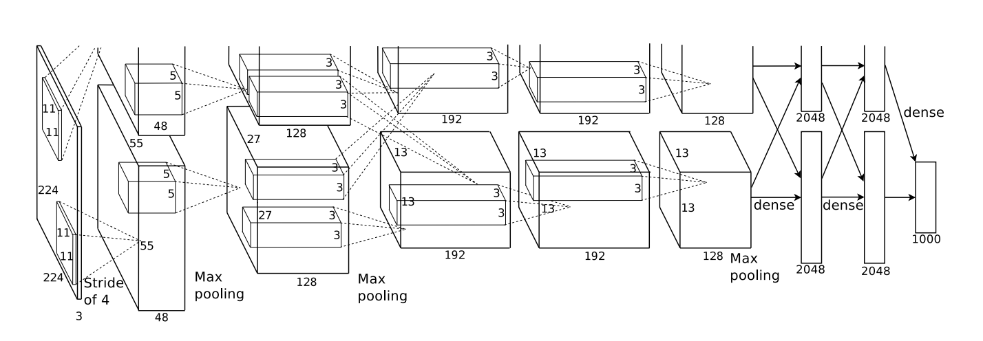
They trained their network to classify images into a thousand different categories.

Randomly guessing, one would guess the correct answer 0.1% of the time. Krizhevsky, et al.’s model is able to give the right answer 63% of the time. Further, one of the top 5 answers it gives is right 85% of the time!

Top: 4 correctly classified examples. Bottom: 4 incorrectly classified examples. Each example has an image, followed by its label, followed by the top 5 guesses with probabilities. From  Krizehvsky et al. (2012).

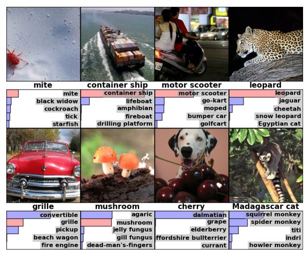
Even some of its errors seem pretty reasonable to me!

We can also examine what the first layer of the network learns to do.

Recall that the convolutional layers were split between the two GPUs. Information doesn’t go back and forth each layer, so the split sides are disconnected in a real way. It turns out that, every time the model is run, the two sides specialize.

Filters learned by the first convolutional layer. The top half corresponds to the layer on one GPU, the bottom on the other. From Krizehvsky et al. (2012)

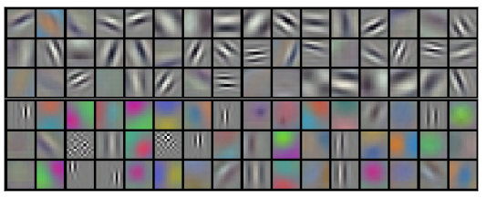
Neurons in one side focus on black and white, learning to detect edges of different orientations and sizes. Neurons on the other side specialize on color and texture, detecting color contrasts and patterns.4 Remember that the neurons are randomly initialized. No human went and set them to be edge detectors, or to split in this way. It arose simply from training the network to classify images.

These remarkable results (and other exciting results around that time) were only the beginning. They were quickly followed by a lot of other work testing modified approaches and gradually improving the results, or applying them to other areas. And, in addition to the neural networks community, many in the computer vision community have adopted deep convolutional neural networks.

Convolutional neural networks are an essential tool in computer vision and modern pattern recognition.

Formalizing Convolutional Neural Networks

Consider a 1-dimensional convolutional layer with inputs  {xn} {xn} and outputs  {yn} {yn}:

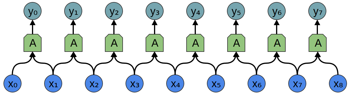
It’s relatively easy to describe the outputs in terms of the inputs:

yn=A(xn,xn+1,...) yn=A(xn,xn+1,...)

For example, in the above:

y0=A(x0,x1) y0=A(x0,x1)

y1=A(x1,x2) y1=A(x1,x2)

Similarly, if we consider a 2-dimensional convolutional layer, with inputs  {xn,m} {xn,m} and outputs  {yn,m} {yn,m}:

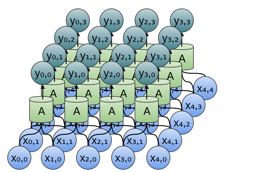
We can, again, write down the outputs in terms of the inputs:

yn,m=A⎛⎝⎜xn, m,xn, m+1,xn+1, m,xn+1, m+1,......, ..., ⎞⎠⎟ yn,m=A(xn, m,xn+1, m,..., xn, m+1,xn+1, m+1,..., ...)

For example:

y0,0=A(x0, 0,x0, 1,x1, 0, x1, 1 ) y0,0=A(x0, 0,x1, 0, x0, 1,x1, 1 )

y1,0=A(x1, 0,x1, 1,x2, 0, x2, 1 ) y1,0=A(x1, 0,x2, 0, x1, 1,x2, 1 )

If one combines this with the equation for  A(x) A(x),

A(x)=σ(Wx+b) A(x)=σ(Wx+b)

one has everything they need to implement a convolutional neural network, at least in theory.

In practice, this is often not best way to think about convolutional neural networks. There is an alternative formulation, in terms of a mathematical operation called convolution, that is often more helpful.

The convolution operation is a powerful tool. In mathematics, it comes up in diverse contexts, ranging from the study of partial differential equations to probability theory. In part because of its role in PDEs, convolution is very important in the physical sciences. It also has an important role in many applied areas, like computer graphics and signal processing.

For us, convolution will provide a number of benefits. Firstly, it will allow us to create much more efficient implementations of convolutional layers than the naive perspective might suggest. Secondly, it will remove a lot of messiness from our formulation, handling all the bookkeeping presently showing up in the indexing of  x xs – the present formulation may not seem messy yet, but that’s only because we haven’t got into the tricky cases yet. Finally, convolution will give us a significantly different perspective for reasoning about convolutional layers.

I admire the elegance of your method of computation; it must be nice to ride through these fields upon the horse of true mathematics while the like of us have to make our way laboriously on foot.  — Albert Einstein

Next Posts in this Series

Read the next post!

This post is part of a series on convolutional neural networks and their generalizations. The first two posts will be review for those familiar with deep learning, while later ones should be of interest to everyone. To get updates, subscribe to my RSS feed!

Please comment below or on the side. Pull requests can be made on github.

Acknowledgments

I’m grateful to Eliana Lorch, Aaron Courville, and Sebastian Zany for their comments and support.

---

1. It should be noted that not all neural networks that use multiple copies of the same neuron are convolutional neural networks. Convolutional neural networks are just one type of neural network that uses the more general trick, weight-tying. Other kinds of neural network that do this are recurrent neural networks and recursive neural networks.↩

2. Groups of neurons, like  A A, that appear in multiple places are sometimes called modules, and networks that use them are sometimes called modular neural networks.↩

3. They also test using 7 in the paper.↩

4. This seems to have interesting analogies to rods and cones in the retina.↩