用R做词云分析

对[文章]1的时候遇到Wordle，根据文章中提示的网址信息，显示为网址打不开。顺藤摸瓜在网上找资料，仍然找不到关于Wordle的online tools，但知道了一本[书]2，其中的一个章节讲解Wordle，指向同样一个网站。我知道是一个强大的工具，必然能够做词云生成，与以”r wordle”和”R 词云”等关键字组合搜索相关资料，最终我将注意力先集中到英文的词云方法，对于中文的词云，要采用特别的处理 （这就想写$\LaTeX$那样，只要你写英文的文章，一切好办，而一牵涉到中文，所做的配置和努力要复杂的多。），最终找到了对我有用的一篇《R做文本挖掘：词云分析》。下面代码主要基于该文，并加上了我自己的感受，因为原文是干巴巴的代码。

在R中画词云图，需要package wordcloud，但是要画出来最终的结果，你需要预先对文档进行必要的分析处理才行，此时需要package tm。再你加载这两包后，系统会自动加载RcolorBrewer和NLP包。在没深入探索之前，我们肯定能猜测出tm就text mining包，而NLP就是自然语言处理包，由此可见R语言功能的强大。

R本身没有默认安装包wordcloud和tm，采用下面代码安装及加载它们：

> install.packages("wordcloud")
> install.packages("tm")
> library(wordcloud)
> library(tm)

有了上面的铺垫工作后，采用下面代码话词云图：

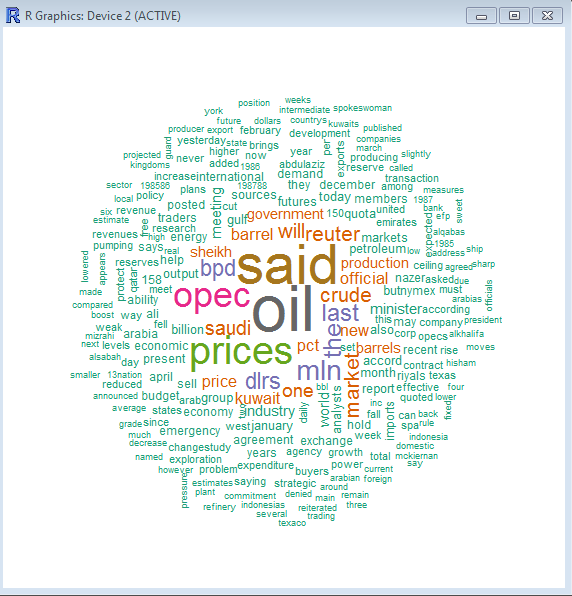
1 采用tm包中的crude数据集画词云图

> data(crude)
> crude <- tm_map(crude,removePunctuation)
> crude <- tm_map(crude,function(x)removeWords(x,stopwords()))
> tdm <- TermDocumentMatrix(crude)
> m <- as.matrix(tdm)
> v <- sort(rowSums(m),decreasing=TRUE)
> d <- data.frame(word=names(v),freq=v)
> wordcloud(d$word,d$freq,random.order=FALSE,colors=brewer.pal(8,"Dark2"))

上面需要一定的R语言语法知识。在此我通俗地讲解一下。先加载数据集crude，对该数据集去标点，去stopwords等后，将其转变成一个矩阵，行为term，列为documents。接下来就好理解了。

最终画好的图如下：

2 采用自定义数据集画词云图

tm包本身已经很强大，能够处理多个文档，当然是对多个文档的所有词来画云图。当然也能处理一个文档，此时termDocument矩阵就变成了一个列向量。现在的问题是你怎么定义自己的数据集？使用tm包中自带的数据集仅仅起到了demo的作用。

首先在如下图所示的路径中建立2个txt文件：

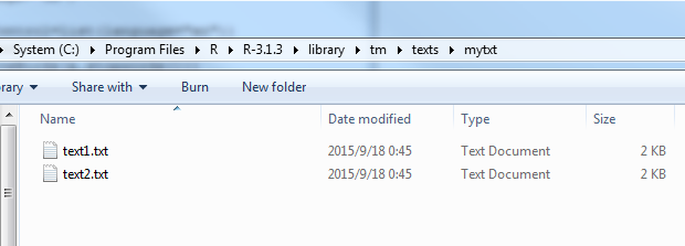
上面C:/Program Files/R/R-3.13/library/tm是R系统tm包的路径。可知，我使用的R版本是3.1.3。接下来，我们就可以画图了。这两个文档的内容分别为：

1. text1.txt

   Most classical search engines choose and rank advertisements (ads) based on their click-through rates (CTRs). To predict an ad’s CTR, historical click information is frequently concerned. To accurately predict the CTR of the new ads is challenging and critical for real world applications, since we do not have plentiful historical data about these ads. Adopting Bayesian network (BN) as the effective framework for representing and inferring dependencies and uncertainties among variables, in this paper, we establish a BN-based model to predict the CTRs of new ads. First, we built a Bayesian network of the keywords that are used to describe the ads in a certain domain, called keyword BN and abbreviated as KBN. Second, we proposed an algorithm for approximate inferences of the KBN to find similar keywords with those that describe the new ads. Finally based on the similar keywords, we obtain the similar ads and then calculate the CTR of the new ad by using the CTRs of the ads that are similar with the new ad. Experimental results show the efficiency and accuracy of our method.

2. text2.txt

   Predicting CTRs for new ads is extremely important and very challenging in the field of computational advertising. In this paper, we proposed an approach for predicting the CTRs of new ads by using the other ads with known CTRs and the inherent similarity of their keywords. The similarity of the ad keywords establishes the similarity of the semantics or functionality of the ads. Adopting BN as the framework for representing and inferring the association and uncertainty, we mainly proposed the methods for constructing and inferring the keyword Bayesian network. Theoretical and experimental results verify the feasibility of our methods.
   To make our methods applicable in realistic situations, we will incorporate the data-intensive computing techniques to improve the efficiency of the aggregation query processing when constructing KBN from the large scale test dataset. Meanwhile, we will also improve the performance of KBN inferences and the corresponding CTR prediction. In this paper, we assume that all the new ad’s keywords are included in the KBN, which is the basis for exploring the method for the situation if not all the keywords are not included (i.e., some keywords of the new ads are missing). Moreover, we can also further explore the accurate user targeting and CTR prediction based on the ideas given in this paper. These are exactly our future work.

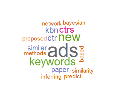
画图命令如下：

txt <- system.file("texts","mytxt",package="tm")
#导入动态coporus
myData <- Corpus(DirSource(txt),readerControl=list(language="en"))
myData <- tm_map(myData,removePunctuation)
myData <- tm_map(myData,function(x)removeWords(x,stopwords()))
tdm <- TermDocumentMatrix(myData)
m <- as.matrix(tdm)
v <- sort(rowSums(m),decreasing=TRUE)
d <- data.frame(word=names(v),freq=v)
wordcloud(d$word,d$freq,random.order=FALSE,color=brewer.pal(8,"Dark2"))

画出的云图的结果为：

关于system.file的更详细的用法及动态coporus的概念，请参见相关的帮助文档。

---

1. Jane Cleland-Huang. Mining Domain Knowledge. IEEE software, 32(3), 2015. ↩
2. Beautiful Visualization Looking at Data Through the Eyes of Experts. Edited by Julie Steele and Noah Iliinsky. O’Reilly, 2010. ↩