Convolutional neural networks(CNN) (九) Implement deep networks for digit classification Exercise

{作为CNN学习入门的一部分，笔者在这里逐步给出UFLDL的各章节Exercise的个人代码实现，供大家参考指正}

理论部分可以在线参阅(页面最下方有中文选项)Self-Taught Learning to Deep Networks到Fine-tuning Stacked AEs部分内容

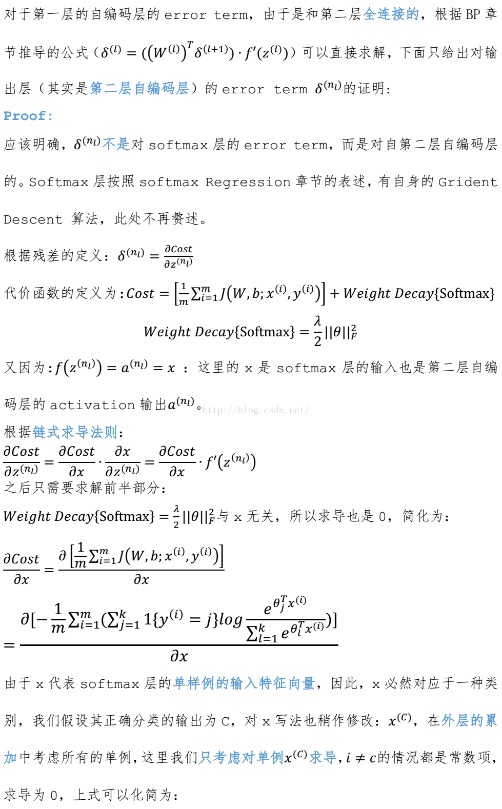
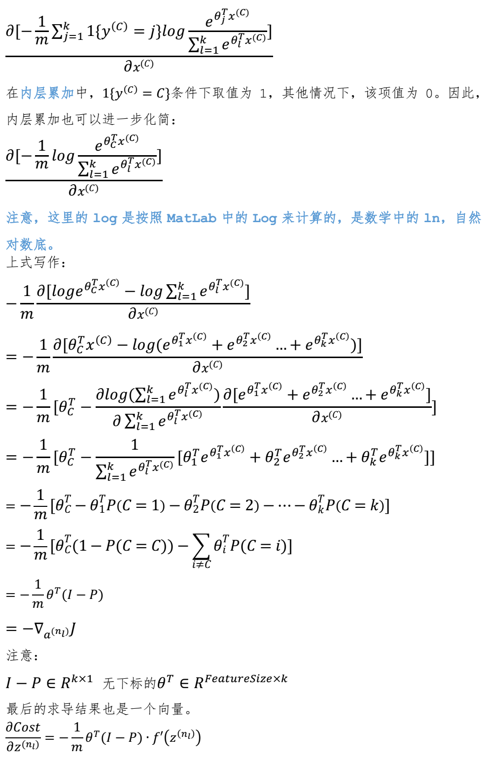
但大部分推导都可以在在线参阅的内容Fine-tuning Stacked AEs中找到，这里只给出对输出层error term求导的证明：

stackedAeCost.m

function [ cost, grad ] = stackedAECost(theta, inputSize, hiddenSize, ...
                                              numClasses, netconfig, ...
                                              lambda, data, labels)
                                         
% stackedAECost: Takes a trained softmaxTheta and a training data set with labels,
% and returns cost and gradient using a stacked autoencoder model. Used for
% finetuning.
                                         
% theta: trained weights from the autoencoder
% visibleSize: the number of input units
% hiddenSize:  the number of hidden units *at the 2nd layer*
% numClasses:  the number of categories
% netconfig:   the network configuration of the stack
% lambda:      the weight regularization penalty
% data: Our matrix containing the training data as columns.  So, data(:,i) is the i-th training example. 
% labels: A vector containing labels, where labels(i) is the label for the
% i-th training example


%% Unroll softmaxTheta parameter

% We first extract the part which compute the softmax gradient
softmaxTheta = reshape(theta(1:hiddenSize*numClasses), numClasses, hiddenSize);

% Extract out the "stack"
stack = params2stack(theta(hiddenSize*numClasses+1:end), netconfig);

% You will need to compute the following gradients
softmaxThetaGrad = zeros(size(softmaxTheta));
stackgrad = cell(size(stack));
for d = 1:numel(stack)
    stackgrad{d}.w = zeros(size(stack{d}.w));
    stackgrad{d}.b = zeros(size(stack{d}.b));
end

% cost = 0; % You need to compute this

% You might find these variables useful
numCases = size(data, 2);
groundTruth = full(sparse(labels, 1:numCases, 1));


%% --------------------------- YOUR CODE HERE -----------------------------
%  Instructions: Compute the cost function and gradient vector for 
%                the stacked autoencoder.
%
%                You are given a stack variable which is a cell-array of
%                the weights and biases for every layer. In particular, you
%                can refer to the weights of Layer d, using stack{d}.w and
%                the biases using stack{d}.b . To get the total number of
%                layers, you can use numel(stack).
%
%                The last layer of the network is connected to the softmax
%                classification layer, softmaxTheta.
%
%                You should compute the gradients for the softmaxTheta,
%                storing that in softmaxThetaGrad. Similarly, you should
%                compute the gradients for each layer in the stack, storing
%                the gradients in stackgrad{d}.w and stackgrad{d}.b
%                Note that the size of the matrices in stackgrad should
%                match exactly that of the size of the matrices in stack.
%                
%                Gradient Check : 1.0932e-11
%

%  ================= Cost =================
%  Stack Layer 
activation_L1 = 1 ./ (1 + exp(-bsxfun(@plus, stack{1}.w*data, stack{1}.b)));
activation_L2 = 1 ./ (1 + exp(-bsxfun(@plus, stack{2}.w*activation_L1, stack{2}.b)));
sae2Features = activation_L2;

%  Softmax Layer
M = softmaxTheta * sae2Features; % M(r,c) is theta.T.r*x(:,c)
M = bsxfun(@minus, M, max(M, [], 1)); % Preventing overflows.
M = exp(M); 
M = bsxfun(@rdivide, M, sum(M)); % Dividing all elements in each column by their column sum.
J_theta = sum(sum(log(M).*groundTruth));
J_theta = -J_theta / numCases;

WeightDecay = lambda * sum(sum(softmaxTheta.^2)) / 2;

cost = J_theta + WeightDecay;

%  ================= Gradient =================
%  Stack Layer
M = groundTruth - M;

Gradient_J = softmaxTheta' * (M);
MatrixDelte_L2 = -Gradient_J/numCases .* activation_L2 .* (1 - activation_L2);
MatrixDelte_L1 = ((stack{2}.w)' * MatrixDelte_L2) .* activation_L1 .* (1 - activation_L1);
stackgrad{1}.w = MatrixDelte_L1 * data';
stackgrad{1}.b = sum(MatrixDelte_L1, 2);
stackgrad{2}.w = MatrixDelte_L2 * activation_L1';
stackgrad{2}.b = sum(MatrixDelte_L2, 2);

%  Softmax Layer

for i = 1:1:numClasses
    softmaxThetaGrad(i,:) = sum(bsxfun(@times, activation_L2, M(i,:)), 2); % Array multiply
end

softmaxThetaGrad = -softmaxThetaGrad/numCases + lambda * softmaxTheta;

% -------------------------------------------------------------------------

%% Roll gradient vector
grad = [softmaxThetaGrad(:) ; stack2params(stackgrad)];

end

stackedAEExercise.m

%% CS294A/CS294W Stacked Autoencoder Exercise

%  Instructions
%  ------------
% 
%  This file contains code that helps you get started on the
%  sstacked autoencoder exercise. You will need to complete code in
%  stackedAECost.m
%  You will also need to have implemented sparseAutoencoderCost.m and 
%  softmaxCost.m from previous exercises. You will need the initializeParameters.m
%  loadMNISTImages.m, and loadMNISTLabels.m files from previous exercises.
%  
%  For the purpose of completing the assignment, you do not need to
%  change the code in this file. 
%
%%======================================================================
%% STEP 0: Here we provide the relevant parameters values that will
%  allow your sparse autoencoder to get good filters; you do not need to 
%  change the parameters below.

inputSize = 28 * 28;
numClasses = 10;
hiddenSizeL1 = 200;    % Layer 1 Hidden Size
hiddenSizeL2 = 200;    % Layer 2 Hidden Size
sparsityParam = 0.1;   % desired average activation of the hidden units.
                       % (This was denoted by the Greek alphabet rho, which looks like a lower-case "p",
		               %  in the lecture notes). 
lambda = 3e-3;         % weight decay parameter       
beta = 3;              % weight of sparsity penalty term    
magnitude = 100;         % magnitude of iteration

%%======================================================================
%% STEP 1: Load data from the MNIST database
%
%  This loads our training data from the MNIST database files.

%  Load MNIST database files
trainData = loadMNISTImages('mnist/train-images.idx3-ubyte');
trainLabels = loadMNISTLabels('mnist/train-labels.idx1-ubyte');

trainLabels(trainLabels == 0) = 10; % Remap 0 to 10 since our labels need to start from 1

%%======================================================================
%% STEP 2: Train the first sparse autoencoder
%  This trains the first sparse autoencoder on the unlabelled STL training
%  images.
%  If you've correctly implemented sparseAutoencoderCost.m, you don't need
%  to change anything here.

%  Randomly initialize the parameters
sae1Theta = initializeParameters(hiddenSizeL1, inputSize);

%% ---------------------- YOUR CODE HERE  ---------------------------------
%  Instructions: Train the first layer sparse autoencoder, this layer has
%                an hidden size of "hiddenSizeL1"
%                You should store the optimal parameters in sae1OptTheta

patches = trainData;

%  Use minFunc to minimize the function
addpath minFunc/
options.Method = 'lbfgs'; % Here, we use L-BFGS to optimize our cost
                          % function. Generally, for minFunc to work, you
                          % need a function pointer with two outputs: the
                          % function value and the gradient. In our problem,
                          % sparseAutoencoderCost.m satisfies this.
options.maxIter = 4 * magnitude;	  % Maximum number of iterations of L-BFGS to run 
options.display = 'on';


[sae1OptTheta, cost] = minFunc( @(p) sparseAutoencoderCost(p, ...
                                   inputSize, hiddenSizeL1, ...
                                   lambda, sparsityParam, ...
                                   beta, patches), ...
                              sae1Theta, options);

% -------------------------------------------------------------------------



%%======================================================================
%% STEP 2: Train the second sparse autoencoder
%  This trains the second sparse autoencoder on the first autoencoder
%  featurse.
%  If you've correctly implemented sparseAutoencoderCost.m, you don't need
%  to change anything here.

[sae1Features] = feedForwardAutoencoder(sae1OptTheta, hiddenSizeL1, ...
                                        inputSize, trainData);

%  Randomly initialize the parameters
sae2Theta = initializeParameters(hiddenSizeL2, hiddenSizeL1);

%% ---------------------- YOUR CODE HERE  ---------------------------------
%  Instructions: Train the second layer sparse autoencoder, this layer has
%                an hidden size of "hiddenSizeL2" and an inputsize of
%                "hiddenSizeL1"
%
%                You should store the optimal parameters in sae2OptTheta

patches = sae1Features;

%  Use minFunc to minimize the function
addpath minFunc/
options.Method = 'lbfgs'; % Here, we use L-BFGS to optimize our cost
                          % function. Generally, for minFunc to work, you
                          % need a function pointer with two outputs: the
                          % function value and the gradient. In our problem,
                          % sparseAutoencoderCost.m satisfies this.
options.maxIter = 4 * magnitude;	  % Maximum number of iterations of L-BFGS to run 
options.display = 'on';


[sae2OptTheta, cost] = minFunc( @(p) sparseAutoencoderCost(p, ...
                                   hiddenSizeL1, hiddenSizeL2, ...
                                   lambda, sparsityParam, ...
                                   beta, patches), ...
                              sae2Theta, options);

% -------------------------------------------------------------------------


%%======================================================================
%% STEP 3: Train the softmax classifier
%  This trains the sparse autoencoder on the second autoencoder features.
%  If you've correctly implemented softmaxCost.m, you don't need
%  to change anything here.

[sae2Features] = feedForwardAutoencoder(sae2OptTheta, hiddenSizeL2, ...
                                        hiddenSizeL1, sae1Features);

%  Randomly initialize the parameters
saeSoftmaxTheta = 0.005 * randn(hiddenSizeL2 * numClasses, 1);


%% ---------------------- YOUR CODE HERE  ---------------------------------
%  Instructions: Train the softmax classifier, the classifier takes in
%                input of dimension "hiddenSizeL2" corresponding to the
%                hidden layer size of the 2nd layer.
%
%                You should store the optimal parameters in saeSoftmaxOptTheta 
%
%  NOTE: If you used softmaxTrain to complete this part of the exercise,
%        set saeSoftmaxOptTheta = softmaxModel.optTheta(:);

lambda = 1e-4;
options.maxIter = 1 * magnitude;
softmaxModel = softmaxTrain(hiddenSizeL2, numClasses, lambda, ...
                            sae2Features, trainLabels, options);
saeSoftmaxOptTheta = softmaxModel.optTheta(:);

% -------------------------------------------------------------------------



%%======================================================================
%% STEP 5: Finetune softmax model

% Implement the stackedAECost to give the combined cost of the whole model
% then run this cell.

% Initialize the stack using the parameters learned
stack = cell(2,1);
stack{1}.w = reshape(sae1OptTheta(1:hiddenSizeL1*inputSize), ...
                     hiddenSizeL1, inputSize);
stack{1}.b = sae1OptTheta(2*hiddenSizeL1*inputSize+1:2*hiddenSizeL1*inputSize+hiddenSizeL1);
stack{2}.w = reshape(sae2OptTheta(1:hiddenSizeL2*hiddenSizeL1), ...
                     hiddenSizeL2, hiddenSizeL1);
stack{2}.b = sae2OptTheta(2*hiddenSizeL2*hiddenSizeL1+1:2*hiddenSizeL2*hiddenSizeL1+hiddenSizeL2);

% Initialize the parameters for the deep model
[stackparams, netconfig] = stack2params(stack);
stackedAETheta = [ saeSoftmaxOptTheta ; stackparams ];

%% ---------------------- YOUR CODE HERE  ---------------------------------
%  Instructions: Train the deep network, hidden size here refers to the '
%                dimension of the input to the classifier, which corresponds 
%                to "hiddenSizeL2".
%
%

[stackedAEOptTheta, cost] =  minFunc( @(p) stackedAECost(p, ...    
                                   inputSize, hiddenSizeL2, ...    
                                   numClasses, netconfig, ...    
                                   lambda, trainData, trainLabels), ...                                       
                              stackedAETheta, options);   
% -------------------------------------------------------------------------



%%======================================================================
%% STEP 6: Test 
%  Instructions: You will need to complete the code in stackedAEPredict.m
%                before running this part of the code
%

% Get labelled test images
% Note that we apply the same kind of preprocessing as the training set
testData = loadMNISTImages('mnist/t10k-images.idx3-ubyte');
testLabels = loadMNISTLabels('mnist/t10k-labels.idx1-ubyte');

testLabels(testLabels == 0) = 10; % Remap 0 to 10

[pred] = stackedAEPredict(stackedAETheta, inputSize, hiddenSizeL2, ...
                          numClasses, netconfig, testData);

acc = mean(testLabels(:) == pred(:));
fprintf('Before Finetuning Test Accuracy: %0.3f%%\n', acc * 100);

[pred] = stackedAEPredict(stackedAEOptTheta, inputSize, hiddenSizeL2, ...
                          numClasses, netconfig, testData);

acc = mean(testLabels(:) == pred(:));
fprintf('After Finetuning Test Accuracy: %0.3f%%\n', acc * 100);

% Accuracy is the proportion of correctly classified images
% The results for our implementation were:
%
% Before Finetuning Test Accuracy: 87.7%
% After Finetuning Test Accuracy:  97.6%
%
% If your values are too low (accuracy less than 95%), you should check 
% your code for errors, and make sure you are training on the 
% entire data set of 60000 28x28 training images 
% (unless you modified the loading code, this should be the case)

stackedAEPredict.m

function [pred] = stackedAEPredict(theta, inputSize, hiddenSize, numClasses, netconfig, data)
                                         
% stackedAEPredict: Takes a trained theta and a test data set,
% and returns the predicted labels for each example.
                                         
% theta: trained weights from the autoencoder
% visibleSize: the number of input units
% hiddenSize:  the number of hidden units *at the 2nd layer*
% numClasses:  the number of categories
% data: Our matrix containing the training data as columns.  So, data(:,i) is the i-th training example. 

% Your code should produce the prediction matrix 
% pred, where pred(i) is argmax_c P(y(c) | x(i)).
 
%% Unroll theta parameter

% We first extract the part which compute the softmax gradient
softmaxTheta = reshape(theta(1:hiddenSize*numClasses), numClasses, hiddenSize);

% Extract out the "stack"
stack = params2stack(theta(hiddenSize*numClasses+1:end), netconfig);

%% ---------- YOUR CODE HERE --------------------------------------
%  Instructions: Compute pred using theta assuming that the labels start 
%                from 1.
activation_L1 = 1 ./ (1 + exp(-bsxfun(@plus, stack{1}.w*data, stack{1}.b)));
activation_L2 = 1 ./ (1 + exp(-bsxfun(@plus, stack{2}.w*activation_L1, stack{2}.b)));
sae2Features = activation_L2;

M = softmaxTheta * sae2Features;
[argmax_c_value_Vec, argmax_c_index_Vec] = max(M, [], 1);
pred = argmax_c_index_Vec;

% -----------------------------------------------------------

end

实验结果：

笔者在实验中采用的迭代轮数为：

两个Sparse AutoEncoder Layer 迭代400次 

Softmax Layer 迭代100次 

Fine-tunning 迭代100次

权重损失系数：

AutoEncoder Layer 3e-3
Softmax Layer 1e-4

Fine-tunning 1e-4

可能由于系数选择的不同以及迭代次数的差异，笔者的实验结果与benchmark有较大差异：

Benchmark为：

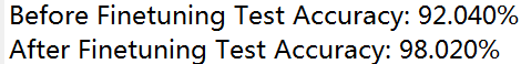
87.7%

97.6%

注：

笔者在softmax层的迭代时，并没有完成100次迭代就达到了精度：

给出大致耗时的估计：

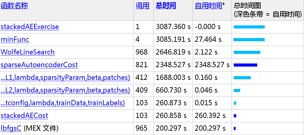
笔者(i7-5500U 16G Maximum Performance)：3087.360/60 = 51.456 mins

Maximum Memory Consumption : About 4.5 GB