R语言关联规则

最新推荐文章于 2022-10-21 19:45:26 发布

程志伟

最新推荐文章于 2022-10-21 19:45:26 发布

阅读量1.1w

点赞数 2

分类专栏： R语言文章标签： r语言

原文链接：https://blog.csdn.net/c1z2w3456789

版权

R语言专栏收录该内容

79 篇文章 38 订阅

订阅专栏

关注微信公共号：小程在线

关注CSDN博客：程志伟的博客

1.概念

1.1 引论

关联规则（AssociationRules）是无监督的机器学习方法，用于知识发现，而非预测。

关联规则的学习器（learner）无需事先对训练数据进行打标签，因为无监督学习没有训练这个步骤。缺点是很难对关联规则学习器进行模型评估，一般都可以通过肉眼观测结果是否合理。

关联规则主要用来发现Pattern，最经典的应用是购物篮分析，当然其他类似于购物篮交易数据的案例也可以应用关联规则进行模式发现，如电影推荐、约会网站或者药物间的相互副作用。

1.2 例子 - 源数据

点击流数据。

不同的Session访问的新闻版块，如下所示：

Session ID	List of media categories accessed
1	{News, Finance}
2	{News, Finance}
3	{Sports, Finance, News}
4	{Arts}
5	{Sports, News, Finance}
6	{News, Arts, Entertainment}

1.3数据格式

关联规则需要把源数据的格式转换为稀疏矩阵。

把上表转化为稀疏矩阵，1表示访问，0表示未访问。

Session ID	News	Finance	Entertainment	Sports
1	1	1	0	0
2	1	1	0	0
3	1	1	0	1
4	0	0	0	0
5	1	1	0	1
6	1	0	1	0

1.4术语和度量

1.4.1项集 ItemSet

这是一条关联规则：

括号内的Item集合称为项集。如上例，{News, Finance}是一个项集，{Sports}也是一个项集。

这个例子就是一条关联规则：基于历史记录，同时看过News和Finance版块的人很有可能会看Sports版块。

{News,Finance} 是这条规则的Left-hand-side (LHS or Antecedent)

{Sports}是这条规则的Right-hand-side (RHS or Consequent)

LHS（Left Hand Side)的项集和RHS（Right Hand Side）的项集不能有交集。

下面介绍衡量关联规则强度的度量。

1.4.2支持度 Support

项集的支持度就是该项集出现的次数除以总的记录数（交易数）。

Support({News}) = 5/6 = 0.83

Support({News, Finance}) = 4/6 =0.67

Support({Sports}) = 2/6 = 0.33

支持度的意义在于度量项集在整个事务集中出现的频次。我们在发现规则的时候，希望关注频次高的项集。

1.4.3置信度 Confidence

关联规则 X -> Y 的置信度计算公式

规则的置信度的意义在于项集{X，Y}同时出现的次数占项集{X}出现次数的比例。发生X的条件下，又发生Y的概率。

表示50%的人访问过{News, Finance}，同时也会访问{Sports}

1.4.4提升度 Lift

当右手边的项集（consequent）的支持度已经很显著时，即时规则的Confidence较高，这条规则也是无效的。

举个例子：

在所分析的10000个事务中,6000个事务包含计算机游戏,7500个包含游戏机游戏,4000个事务同时包含两者。

关联规则（计算机游戏，游戏机游戏）支持度为0.4，看似很高，但其实这个关联规则是一个误导。

在用户购买了计算机游戏后有（4000÷6000）0.667 的概率的去购买游戏机游戏，而在没有任何前提条件时，用户反而有（7500÷10000）0.75的概率去购买游戏机游戏，也就是说设置了购买计算机游戏这样的条件反而会降低用户去购买游戏机游戏的概率，所以计算机游戏和游戏机游戏是相斥的。

所以要引进Lift这个概念，Lift(X->Y)=Confidence(X->Y)/Support(Y)

规则的提升度的意义在于度量项集{X}和项集{Y}的独立性。即，Lift(X->Y)= 1 表面 {X}，{Y}相互独立。[注：P(XY)=P(X)*P(Y),if X is independent of Y]

如果该值=1,说明两个条件没有任何关联,如果<1,说明A条件(或者说A事件的发生)与B事件是相斥的,一般在数据挖掘中当提升度大于3时,我们才承认挖掘出的关联规则是有价值的。

最后，lift(X->Y) = lift(Y->X)

1.4.5出错率 Conviction

Conviction的意义在于度量规则预测错误的概率。

表示X出现而Y不出现的概率。

例子：

表面这条规则的出错率是32%。

1.5生成规则

一般两步：

第一步，找出频繁项集。n个item，可以产生2^n- 1 个项集（itemset）。所以，需要指定最小支持度，用于过滤掉非频繁项集。
第二部，找出第一步的频繁项集中的规则。n个item，总共可以产生3^n - 2^(n+1) + 1条规则。所以，需要指定最小置信度，用于过滤掉弱规则。

第一步的计算量比第二部的计算量大。

2.Apriori算法

Apriori Principle

如果项集A是频繁的，那么它的子集都是频繁的。如果项集A是不频繁的，那么所有包括它的父集都是不频繁的。

例子：{X, Y}是频繁的，那么{X}，{Y}也是频繁的。如果{Z}是不频繁的，那么{X,Z}, {Y, Z}, {X, Y, Z}都是不频繁的。

生成频繁项集

给定最小支持度Sup，计算出所有大于等于Sup的项集。

第一步，计算出单个item的项集，过滤掉那些不满足最小支持度的项集。

第二步，基于第一步，生成两个item的项集，过滤掉那些不满足最小支持度的项集。

第三步，基于第二步，生成三个item的项集，过滤掉那些不满足最小支持度的项集。

如下例子：

One-Item Sets	Support Count	Support
{News}	5	0.83
{Finance}	4	0.67
{Entertainment}	1	0.17
{Sports}	2	0.33
Two-Item Sets	Support Count	Support
{News, Finance}	4	0.67
{News, Sports}	2	0.33
{Finance, Sports}	2	0.33
Three-Item Sets	Support Count	Support
{News, Finance, Sports}	2	0.33

规则生成

给定Confidence、Lift 或者 Conviction，基于上述生成的频繁项集，生成规则，过滤掉那些不满足目标度量的规则。因为规则相关的度量都是通过支持度计算得来，所以这部分过滤的过程很容易完成。

Apriori案例分析（R语言）

1. 关联规则的包

arules是用来进行关联规则分析的R语言包。

[java] view plain copy

print ?

library(arules)

2. 加载数据集

源数据：groceries 数据集，每一行代表一笔交易所购买的产品（item）

数据转换：创建稀疏矩阵，每个Item一列，每一行代表一个transaction。1表示该transaction购买了该item，0表示没有购买。当然，data frame是比较直观的一种数据结构，但是一旦item比较多的时候，这个data frame的大多数单元格的值为0，大量浪费内存。所以，R引入了特殊设计的稀疏矩阵，仅存1，节省内存。arules包的函数read.transactions可以读入源数据并创建稀疏矩阵。

[java] view plain copy

print ?

groceries <- read.transactions("groceries.csv", format="basket", sep=",")

参数说明：

format=c("basket", "single")用于注明源数据的格式。如果源数据每行内容就是一条交易购买的商品列表（类似于一行就是一个购物篮）那么使用basket；如果每行内容是交易号+单个商品，那么使用single。

cols=c("transId", "ItemId") 对于single格式，需要指定cols，二元向量（数字或字符串）。如果是字符串，那么文件的第一行是表头（即列名）。第一个元素是交易号的字段名，第二个元素是商品编号的字段名。如果是数字，那么无需表头。对于basket，一般设置为NULL，缺省也是NULL，所以不用指定。

signle format的数据格式如下所示，与此同时，需要设定cols=c(1, 2)

1001,Fries

1001,Coffee

1001,Milk

1002,Coffee

1002,Fries

rm.duplicates=FALSE：表示对于同一交易，是否需要删除重复的商品。

接下来，查看数据集相关的统计汇总信息，以及数据集本身。

[java] view plain copy

print ?

summary(groceries)
transactions as itemMatrix in sparse format with
9835 rows (elements/itemsets/transactions) and
169 columns (items) and a density of 0.02609146
most frequent items:
whole milk other vegetables rolls/buns soda
2513 1903 1809 1715
yogurt (Other)
1372 34055
element (itemset/transaction) length distribution:
sizes
1 2 3 4 5 6 7 8 9 10 11 12 13 14 15
2159 1643 1299 1005 855 645 545 438 350 246 182 117 78 77 55
16 17 18 19 20 21 22 23 24 26 27 28 29 32
46 29 14 14 9 11 4 6 1 1 1 1 3 1
Min. 1st Qu. Median Mean 3rd Qu. Max.
1.000 2.000 3.000 4.409 6.000 32.000
includes extended item information - examples:
labels
1 abrasive cleaner
2 artif. sweetener
3 baby cosmetics

summary的含义：

第一段：总共有9835条交易记录transaction，169个商品item。density=0.026表示在稀疏矩阵中1的百分比。
第二段：最频繁出现的商品item，以及其出现的次数。可以计算出最大支持度。

第三段：每笔交易包含的商品数目，以及其对应的5个分位数和均值的统计信息。如：2159条交易仅包含了1个商品，1643条交易购买了2件商品，一条交易购买了32件商品。那段统计信息的含义是：第一分位数是2，意味着25%的交易包含不超过2个item。中位数是3表面50%的交易购买的商品不超过3件。均值4.4表示所有的交易平均购买4.4件商品。

第四段：如果数据集包含除了Transaction Id 和 Item之外的其他的列（如，发生交易的时间，用户ID等等），会显示在这里。这个例子，其实没有新的列，labels就是item的名字。

进一步查看数据集的信息

[java] view plain copy

print ?

> class(groceries)
[1] "transactions"
attr(,"package")
[1] "arules"
> groceries
transactions in sparse format with
9835 transactions (rows) and
169 items (columns)
> dim(groceries)
[1] 9835 169
> colnames(groceries)[1:5]
[1] "abrasive cleaner" "artif. sweetener" "baby cosmetics" "baby food" "bags"
> rownames(groceries)[1:5]
[1] "1" "2" "3" "4" "5"

basketSize表示每个transaction包含item的数目，是row level。而ItemFrequency是这个item的支持度，是column level。

[java] view plain copy

print ?

> basketSize<-size(groceries)
> summary(basketSize)
Min. 1st Qu. Median Mean 3rd Qu. Max.
1.000 2.000 3.000 4.409 6.000 32.000
> sum(basketSize) #count of all 1s in the sparse matrix
[1] 43367
> itemFreq <- itemFrequency(groceries)
> itemFreq[1:5]
abrasive cleaner artif. sweetener baby cosmetics baby food bags
0.0035587189 0.0032536858 0.0006100661 0.0001016777 0.0004067107
> sum(itemFreq) #本质上代表"平均一个transaction购买的item个数"
[1] 4.409456

可以查看basketSize的分布：密度曲线(TO ADD HERE)

itemCount表示每个item出现的次数。Support(X) = Xs / N, N是总的交易数，Xs就是Item X的count。

itemXCount = N * itemXFreq = (ItemXFreq / sum(itemFreq)) * sum(basketSize)

[java] view plain copy

print ?

> itemCount <- (itemFreq/sum(itemFreq))*sum(basketSize)
> summary(itemCount)
Min. 1st Qu. Median Mean 3rd Qu. Max.
1.0 38.0 103.0 256.6 305.0 2513.0
> orderedItem <- sort(itemCount, decreasing = )
> orderedItem <- sort(itemCount, decreasing = T)
> orderedItem[1:10]
whole milk other vegetables rolls/buns soda yogurt bottled water
2513 1903 1809 1715 1372 1087
root vegetables tropical fruit shopping bags sausage
1072 1032 969 924

当然，也可以把支持度itemFrequency排序，查看支持度的最大值

[java] view plain copy

print ?

> orderedItemFreq <- sort(itemFrequency(groceries), decreasing=T)
> orderedItemFreq[1:10]
whole milk other vegetables rolls/buns soda yogurt bottled water
0.25551601 0.19349263 0.18393493 0.17437722 0.13950178 0.11052364
root vegetables tropical fruit shopping bags sausage
0.10899847 0.10493137 0.09852567 0.09395018

如果要切一块子集出来计算支持度，可以对数据集进行矩阵行列下标操作。

如下例，切除第100行到800行，计算第1列到第3列的支持度。也就是说，数据集通过向量的下标按行切，也可以通过矩阵下标按行列切。

[java] view plain copy

print ?

> itemFrequency(groceries[100:800,1:3])
abrasive cleaner artif. sweetener baby cosmetics
0.005706134 0.001426534 0.001426534

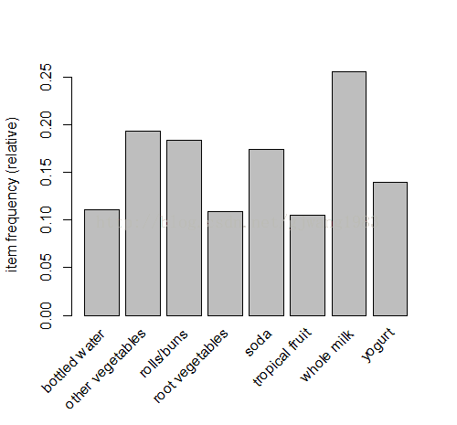
可以通过图形更直观观测。

按最小支持度查看。

[java] view plain copy

print ?

> itemFrequencyPlot(groceries, support=0.1)

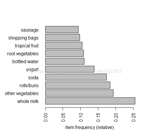
按照排序查看。

[java] view plain copy

print ?

> itemFrequencyPlot(groceries, topN=10, horiz=T)

最后，可以根据业务对数据集进行过滤，获得进一步规则挖掘的数据集。如下例，只关心购买两件商品以上的交易。

[java] view plain copy

print ?

> groceries_use <- groceries[basketSize > 1]
> dim(groceries_use)
[1] 7676 169

查看数据

[java] view plain copy

print ?

inspect(groceries[1:5])
items
1 {citrus fruit,
margarine,
ready soups,
semi-finished bread}
2 {coffee,
tropical fruit,
yogurt}
3 {whole milk}
4 {cream cheese,
meat spreads,
pip fruit,
yogurt}
5 {condensed milk,
long life bakery product,
other vegetables,
whole milk}

也可以通过图形更直观观测数据的稀疏情况。一个点代表在某个transaction上购买了item。

[java] view plain copy

print ?

> image(groceries[1:10])

当数据集很大的时候，这张稀疏矩阵图是很难展现的，一般可以用sample函数进行采样显示。

[java] view plain copy

print ?

> image(sample(groceries,100))

这个矩阵图虽然看上去没有包含很多信息，但是它对于直观地发现异常数据或者比较特殊的Pattern很有效。比如，某些item几乎每个transaction都会买。比如，圣诞节都会买糖果礼物。那么在这幅图上会显示一根竖线，在糖果这一列上。

给出一个通用的R函数，用于显示如上所有的指标：

<a target=_blank id="L1" href="http://blog.csdn.net/gjwang1983/article/details/45015203#L1" rel="#L1" style="color: rgb(102, 102, 102); text-decoration: none;"> 1</a>
<a target=_blank id="L2" href="http://blog.csdn.net/gjwang1983/article/details/45015203#L2" rel="#L2" style="color: rgb(102, 102, 102); text-decoration: none;"> 2</a>
<a target=_blank id="L3" href="http://blog.csdn.net/gjwang1983/article/details/45015203#L3" rel="#L3" style="color: rgb(102, 102, 102); text-decoration: none;"> 3</a>

library(arules) # association rules

library(arulesViz) # data visualization of association rules

library(RColorBrewer) # color palettes for plots

来自CODE的代码片

apriori.R

3. 进行规则挖掘

为了进行规则挖掘，第一步是设定一个最小支持度，这个最小支持度可以由具体的业务规则确定。

介绍apriori函数的用法：

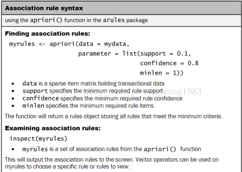
这里需要说明下parameter：

默认的support=0.1, confidence=0.8, minlen=1, maxlen=10

对于minlen，maxlen这里指规则的LHS+RHS的并集的元素个数。所以minlen=1，意味着 {} => {beer}是合法的规则。我们往往不需要这种规则，所以需要设定minlen=2。

[java] view plain copy

print ?

> groceryrules <- apriori(groceries, parameter = list(support =
+ 0.006, confidence = 0.25, minlen = 2))
Parameter specification:
confidence minval smax arem aval originalSupport support minlen maxlen target ext
0.25 0.1 1 none FALSE TRUE 0.006 2 10 rules FALSE
Algorithmic control:
filter tree heap memopt load sort verbose
0.1 TRUE TRUE FALSE TRUE 2 TRUE
apriori - find association rules with the apriori algorithm
version 4.21 (2004.05.09) (c) 1996-2004 Christian Borgelt
set item appearances ...[0 item(s)] done [0.00s].
set transactions ...[169 item(s), 9835 transaction(s)] done [0.00s].
sorting and recoding items ... [109 item(s)] done [0.00s].
creating transaction tree ... done [0.00s].
checking subsets of size 1 2 3 4 done [0.01s].
writing ... [463 rule(s)] done [0.00s].
creating S4 object ... done [0.00s].

从返回的结果看，总共有463条规则生成。

评估模型

使用summary函数查看规则的汇总信息。

[java] view plain copy

print ?

> summary(groceryrules)
set of 463 rules
rule length distribution (lhs + rhs):sizes
2 3 4
150 297 16
Min. 1st Qu. Median Mean 3rd Qu. Max.
2.000 2.000 3.000 2.711 3.000 4.000
summary of quality measures:
support confidence lift
Min. :0.006101 Min. :0.2500 Min. :0.9932
1st Qu.:0.007117 1st Qu.:0.2971 1st Qu.:1.6229
Median :0.008744 Median :0.3554 Median :1.9332
Mean :0.011539 Mean :0.3786 Mean :2.0351
3rd Qu.:0.012303 3rd Qu.:0.4495 3rd Qu.:2.3565
Max. :0.074835 Max. :0.6600 Max. :3.9565
mining info:
data ntransactions support confidence
groceries 9835 0.006 0.25

第一部分：规则的长度分布：就是minlen到maxlen之间的分布。如上例，len=2有150条规则，len=3有297，len=4有16。同时，rule length的五数分布+均值。

第二部分：quality measure的统计信息。

第三部分：挖掘的相关信息。

使用inpect查看具体的规则。

[java] view plain copy

print ?

> inspect(groceryrules[1:5])
lhs rhs support confidence lift
1 {potted plants} => {whole milk} 0.006914082 0.4000000 1.565460
2 {pasta} => {whole milk} 0.006100661 0.4054054 1.586614
3 {herbs} => {root vegetables} 0.007015760 0.4312500 3.956477
4 {herbs} => {other vegetables} 0.007727504 0.4750000 2.454874
5 {herbs} => {whole milk} 0.007727504 0.4750000 1.858983

4. 评估规则

规则可以划分为3大类：

Actionable
- 这些rule提供了非常清晰、有用的洞察，可以直接应用在业务上。

Trivial
- 这些rule显而易见，很清晰但是没啥用。属于common sense，如 {尿布} => {婴儿食品}。

Inexplicable
- 这些rule是不清晰的，难以解释，需要额外的研究来判定是否是有用的rule。

接下来，我们讨论如何发现有用的rule。

按照某种度量，对规则进行排序。

[java] view plain copy

print ?

> ordered_groceryrules <- sort(groceryrules, by="lift")
> inspect(ordered_groceryrules[1:5])
lhs rhs support confidence lift
1 {herbs} => {root vegetables} 0.007015760 0.4312500 3.956477
2 {berries} => {whipped/sour cream} 0.009049314 0.2721713 3.796886
3 {other vegetables,
tropical fruit,
whole milk} => {root vegetables} 0.007015760 0.4107143 3.768074
4 {beef,
other vegetables} => {root vegetables} 0.007930859 0.4020619 3.688692
5 {other vegetables,
tropical fruit} => {pip fruit} 0.009456024 0.2634561 3.482649

搜索规则

[java] view plain copy

print ?

> yogurtrules <- subset(groceryrules, items %in% c("yogurt"))
> inspect(yogurtrules)
lhs rhs support confidence lift
1 {cat food} => {yogurt} 0.006202339 0.2663755 1.909478
2 {hard cheese} => {yogurt} 0.006405694 0.2614108 1.873889
3 {butter milk} => {yogurt} 0.008540925 0.3054545 2.189610
......
18 {cream cheese,
yogurt} => {whole milk} 0.006609049 0.5327869 2.085141
......
121 {other vegetables,
whole milk} => {yogurt} 0.022267412 0.2975543 2.132979

items %in% c("A", "B")表示 lhs+rhs的项集并集中，至少有一个item是在c("A", "B")。 item = Aor item = B

如果仅仅想搜索lhs或者rhs，那么用lhs或rhs替换items即可。如：lhs %in% c("yogurt")

%in%是精确匹配

%pin%是部分匹配，也就是说只要item like '%A%' or item like '%B%'

%ain%是完全匹配，也就是说itemset has ’A' and itemset has ‘B'

同时可以通过条件运算符(&, |, !) 添加 support, confidence, lift的过滤条件。

例子如下：

[java] view plain copy

print ?

> fruitrules <- subset(groceryrules, items %pin% c("fruit"))
> inspect(fruitrules)
lhs rhs support confidence lift
1 {grapes} => {tropical fruit} 0.006100661 0.2727273 2.599101
2 {fruit/vegetable juice} => {soda} 0.018403660 0.2545710 1.459887

[java] view plain copy

print ?

> byrules <- subset(groceryrules, items %ain% c("berries", "yogurt"))
> inspect(byrules)
lhs rhs support confidence lift
1 {berries} => {yogurt} 0.01057448 0.3180428 2.279848

[java] view plain copy

print ?

> fruitrules <- subset(groceryrules, items %pin% c("fruit") & lift > 2)
> inspect(fruitrules)
lhs rhs support confidence lift
1 {grapes} => {tropical fruit} 0.006100661 0.2727273 2.599101
2 {pip fruit} => {tropical fruit} 0.020437214 0.2701613 2.574648
3 {tropical fruit} => {yogurt} 0.029283172 0.2790698 2.000475
4 {curd,
tropical fruit} => {whole milk} 0.006507372 0.6336634 2.479936
5 {butter,
tropical fruit} => {whole milk} 0.006202339 0.6224490 2.436047

查看其它的quality measure

[java] view plain copy

print ?

<pre name="code" class="java">> qualityMeasures <- interestMeasure(groceryrules, method=c("coverage","fishersExactTest","conviction", "chiSquared"), transactions=groceries)
> summary(qualityMeasures)
coverage fishersExactTest conviction chiSquared
Min. :0.009964 Min. :0.0000000 Min. :0.9977 Min. : 0.0135
1st Qu.:0.018709 1st Qu.:0.0000000 1st Qu.:1.1914 1st Qu.: 32.1179
Median :0.024809 Median :0.0000000 Median :1.2695 Median : 58.4354
Mean :0.032608 Mean :0.0057786 Mean :1.3245 Mean : 70.4249
3rd Qu.:0.035892 3rd Qu.:0.0000001 3rd Qu.:1.4091 3rd Qu.: 97.1387
Max. :0.255516 Max. :0.5608331 Max. :2.1897 Max. :448.5699
> quality(groceryrules) <- cbind(quality(groceryrules), qualityMeasures)
> inspect(head(sort(groceryrules, by = "conviction", decreasing = F)))
lhs rhs support confidence lift conviction chiSquared coverage fishersExactTest
1 {bottled beer} => {whole milk} 0.020437214 0.2537879 0.9932367 0.9976841 0.01352288 0.08052872 0.5608331
2 {bottled water,
soda} => {whole milk} 0.007524148 0.2596491 1.0161755 1.0055826 0.02635700 0.02897814 0.4586202
3 {beverages} => {whole milk} 0.006812405 0.2617188 1.0242753 1.0084016 0.05316028 0.02602949 0.4329533
4 {specialty chocolate} => {whole milk} 0.008032537 0.2642140 1.0340410 1.0118214 0.12264445 0.03040163 0.3850343
5 {candy} => {whole milk} 0.008235892 0.2755102 1.0782502 1.0275976 0.63688634 0.02989324 0.2311769
6 {sausage,
soda} => {whole milk} 0.006710727 0.2761506 1.0807566 1.0285068 0.54827850 0.02430097 0.2508610

第三个参数transactions：一般情况下都是原来那个数据集，但也有可能是其它数据集，用于检验这些rules在其他数据集上的效果。所以，这也是评估rules的一种方法：在其它数据集上计算这些规则的quality measure用以评估效果。

fishersExactTest 的p值大部分都是很小的（p < 0.05），这就说明这些规则反应出了真实的用户的行为模式。

coverage从0.01 ~ 0.26，相当于覆盖到了多少范围的用户。

ChiSquared: 考察该规则的LHS和RHS是否独立？即LHS与RHS的列联表的ChiSquare Test。p<0.05表示独立，否则表示不独立。

限制挖掘的item

可以控制规则的左手边或者右手边出现的item，即appearance。但尽量要放低支持度和置信度。

[java] view plain copy

print ?

> berriesInLHS <- apriori(groceries, parameter = list( support = 0.001, confidence = 0.1 ), appearance = list(lhs = c("berries"), default="rhs"))
Parameter specification:
confidence minval smax arem aval originalSupport support minlen maxlen target ext
0.1 0.1 1 none FALSE TRUE 0.001 1 10 rules FALSE
Algorithmic control:
filter tree heap memopt load sort verbose
0.1 TRUE TRUE FALSE TRUE 2 TRUE
apriori - find association rules with the apriori algorithm
version 4.21 (2004.05.09) (c) 1996-2004 Christian Borgelt
set item appearances ...[1 item(s)] done [0.00s].
set transactions ...[169 item(s), 9835 transaction(s)] done [0.00s].
sorting and recoding items ... [157 item(s)] done [0.00s].
creating transaction tree ... done [0.00s].
checking subsets of size 1 2 done [0.00s].
writing ... [26 rule(s)] done [0.00s].
creating S4 object ... done [0.00s].
> summary(berriesInLHS)
set of 26 rules
rule length distribution (lhs + rhs):sizes
1 2
8 18
Min. 1st Qu. Median Mean 3rd Qu. Max.
1.000 1.000 2.000 1.692 2.000 2.000
summary of quality measures:
support confidence lift
Min. :0.003660 Min. :0.1049 Min. :1.000
1st Qu.:0.004601 1st Qu.:0.1177 1st Qu.:1.000
Median :0.007016 Median :0.1560 Median :1.470
Mean :0.053209 Mean :0.1786 Mean :1.547
3rd Qu.:0.107982 3rd Qu.:0.2011 3rd Qu.:1.830
Max. :0.255516 Max. :0.3547 Max. :3.797
mining info:
data ntransactions support confidence
groceries 9835 0.001 0.1
> inspect(berriesInLHS)
lhs rhs support confidence lift
1 {} => {bottled water} 0.110523640 0.1105236 1.000000
2 {} => {tropical fruit} 0.104931368 0.1049314 1.000000
3 {} => {root vegetables} 0.108998475 0.1089985 1.000000
4 {} => {soda} 0.174377224 0.1743772 1.000000
5 {} => {yogurt} 0.139501779 0.1395018 1.000000
6 {} => {rolls/buns} 0.183934926 0.1839349 1.000000
7 {} => {other vegetables} 0.193492628 0.1934926 1.000000
8 {} => {whole milk} 0.255516014 0.2555160 1.000000
9 {berries} => {beef} 0.004473818 0.1345566 2.564659
10 {berries} => {butter} 0.003762074 0.1131498 2.041888
11 {berries} => {domestic eggs} 0.003863752 0.1162080 1.831579
12 {berries} => {fruit/vegetable juice} 0.003660397 0.1100917 1.522858
13 {berries} => {whipped/sour cream} 0.009049314 0.2721713 3.796886
14 {berries} => {pip fruit} 0.003762074 0.1131498 1.495738
15 {berries} => {pastry} 0.004270463 0.1284404 1.443670
16 {berries} => {citrus fruit} 0.005388917 0.1620795 1.958295
17 {berries} => {shopping bags} 0.004982206 0.1498471 1.520894
18 {berries} => {sausage} 0.004982206 0.1498471 1.594963
19 {berries} => {bottled water} 0.004067107 0.1223242 1.106769
20 {berries} => {tropical fruit} 0.006710727 0.2018349 1.923494
21 {berries} => {root vegetables} 0.006609049 0.1987768 1.823666
22 {berries} => {soda} 0.007320793 0.2201835 1.262685
23 {berries} => {yogurt} 0.010574479 0.3180428 2.279848
24 {berries} => {rolls/buns} 0.006609049 0.1987768 1.080691
25 {berries} => {other vegetables} 0.010269446 0.3088685 1.596280
26 {berries} => {whole milk} 0.011794611 0.3547401 1.388328

既然lhs都是一样的，那么只查看rhs的itemset即可，可以如下：

[java] view plain copy

print ?

> inspect(head(rhs(berriesInLHS), n=5))
items
1 {bottled water}
2 {tropical fruit}
3 {root vegetables}
4 {soda}
5 {yogurt}

当然，还可以使用subset进行进一步的过滤，例如，不希望看到rhs包含"root vegetables" 或 "whole milk"

[java] view plain copy

print ?

> berrySub <- subset(berriesInLHS, subset = !(rhs %in% c("root vegetables", "whole milk")))
> inspect(head(rhs(sort(berrySub, by="confidence")), n=5))
items
1 {yogurt}
2 {other vegetables}
3 {whipped/sour cream}
4 {soda}
5 {tropical fruit}
> berrySub
set of 22 rules

保存挖掘的结果

有两种使用场景。

第一，保存到文件。可以与外部程序进行交换。

[java] view plain copy

print ?

> write(groceryrules, file="groceryrules.csv", sep=",", quote=TRUE, row.names=FALSE)

第二，转换为data frame，然后再进行进一步的处理。处理完的结果可以保存到外部文件或者数据库。

[java] view plain copy

print ?

> groceryrules_df <- as(groceryrules, "data.frame")
> str(groceryrules_df)
'data.frame': 463 obs. of 8 variables:
$ rules : Factor w/ 463 levels "{baking powder} => {other vegetables}",..: 340 302 207 206 208 341 402 21 139 140 ...
$ support : num 0.00691 0.0061 0.00702 0.00773 0.00773 ...
$ confidence : num 0.4 0.405 0.431 0.475 0.475 ...
$ lift : num 1.57 1.59 3.96 2.45 1.86 ...
$ conviction : num 1.24 1.25 1.57 1.54 1.42 ...
$ chiSquared : num 19 17.7 173.9 82.6 41.2 ...
$ coverage : num 0.0173 0.015 0.0163 0.0163 0.0163 ...
$ fishersExactTest: num 2.20e-05 4.13e-05 6.17e-26 4.56e-16 1.36e-09 ...

关于关联规则挖掘的进阶部分

1. 带有Hierarchy的item

这里我们使用arules自带的数据集Groceries。该数据集不仅包含购物篮的item信息，而且还包含每个item对于的类别，总共有两层类别。如下所示：

[java] view plain copy

print ?

> data(Groceries) # grocery transactions object from arules package
>
> summary(Groceries)
transactions as itemMatrix in sparse format with
9835 rows (elements/itemsets/transactions) and
169 columns (items) and a density of 0.02609146
most frequent items:
whole milk other vegetables rolls/buns soda yogurt (Other)
2513 1903 1809 1715 1372 34055
element (itemset/transaction) length distribution:
sizes
1 2 3 4 5 6 7 8 9 10 11 12 13 14 15 16 17 18 19 20 21 22 23 24 26 27 28 29 32
2159 1643 1299 1005 855 645 545 438 350 246 182 117 78 77 55 46 29 14 14 9 11 4 6 1 1 1 1 3 1
Min. 1st Qu. Median Mean 3rd Qu. Max.
1.000 2.000 3.000 4.409 6.000 32.000
includes extended item information - examples:
labels level2 level1
1 frankfurter sausage meet and sausage
2 sausage sausage meet and sausage
3 liver loaf sausage meet and sausage

在summary的最后一部分，我们发现除了labels（即item）之外，还有两个字段，level2和level1。我们可以通过itemInfo进行查看level1和level2的详细信息，如下所示：

[java] view plain copy

print ?

> print(levels(itemInfo(Groceries)[["level1"]]))
[1] "canned food" "detergent" "drinks" "fresh products" "fruit and vegetables" "meet and sausage" "non-food"
[8] "perfumery" "processed food" "snacks and candies"
> print(levels(itemInfo(Groceries)[["level2"]]))
[1] "baby food" "bags" "bakery improver" "bathroom cleaner"
[5] "beef" "beer" "bread and backed goods" "candy"
[9] "canned fish" "canned fruit/vegetables" "cheese" "chewing gum"
[13] "chocolate" "cleaner" "coffee" "condiments"
[17] "cosmetics" "dairy produce" "delicatessen" "dental care"
[21] "detergent/softener" "eggs" "fish" "frozen foods"
[25] "fruit" "games/books/hobby" "garden" "hair care"
[29] "hard drinks" "health food" "jam/sweet spreads" "long-life bakery products"
[33] "meat spreads" "non-alc. drinks" "non-food house keeping products" "non-food kitchen"
[37] "packaged fruit/vegetables" "perfumery" "personal hygiene" "pet food/care"
[41] "pork" "poultry" "pudding powder" "sausage"
[45] "seasonal products" "shelf-stable dairy" "snacks" "soap"
[49] "soups/sauces" "staple foods" "sweetener" "tea/cocoa drinks"
[53] "vegetables" "vinegar/oils" "wine"

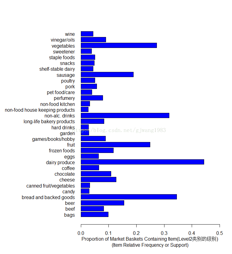
一般来说，如果商品有类别信息，可以尝试在类别上进行关联规则的挖掘，毕竟成千上百个商品之间的规则挖掘要困难得多。可以先从高粒度上进行挖掘实验，然后再进行细粒度的挖掘实验。本例中，因为Level1包含的类别信息太少，关联规则的挖掘没有意义，而Level2有55个，可以使用Level2。在R中，可以用aggregate函数把item替换为它对应的category，如下所示：（可以把aggregate看成transform的过程）

[java] view plain copy

print ?

> inspect(Groceries[1:3])
items
1 {citrus fruit,
semi-finished bread,
margarine,
ready soups}
2 {tropical fruit,
yogurt,
coffee}
3 {whole milk}
> groceries <- aggregate(Groceries, itemInfo(Groceries)[["level2"]])
> inspect(groceries[1:3])
items
1 {bread and backed goods,
fruit,
soups/sauces,
vinegar/oils}
2 {coffee,
dairy produce,
fruit}
3 {dairy produce}

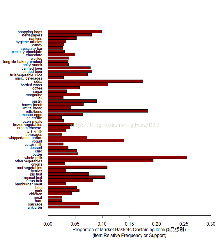
我们可以对比一下在aggregate前后的itemFrequency图。

[java] view plain copy

print ?

itemFrequencyPlot(Groceries, support = 0.025, cex.names=0.8, xlim = c(0,0.3),
type = "relative", horiz = TRUE, col = "dark red", las = 1,
xlab = paste("Proportion of Market Baskets Containing Item",
"\n(Item Relative Frequency or Support)"))

[java] view plain copy

print ?

horiz=TRUE: 让柱状图水平显示

[java] view plain copy

print ?

cex.names=0.8:item的label（这个例子即纵轴）的大小乘以的系数。

[java] view plain copy

print ?

las=1: 表示刻度的方向，1表示总是水平方向。

[java] view plain copy

print ?

type="relative": 即support的值（百分比）。如果type=absolute表示显示该item的count，而非support。默认就是relative。

2. 规则的图形展现

假设我们有这样一个规则集合：

[java] view plain copy

print ?

> second.rules <- apriori(groceries,
+ parameter = list(support = 0.025, confidence = 0.05))
Parameter specification:
confidence minval smax arem aval originalSupport support minlen maxlen target ext
0.05 0.1 1 none FALSE TRUE 0.025 1 10 rules FALSE
Algorithmic control:
filter tree heap memopt load sort verbose
0.1 TRUE TRUE FALSE TRUE 2 TRUE
apriori - find association rules with the apriori algorithm
version 4.21 (2004.05.09) (c) 1996-2004 Christian Borgelt
set item appearances ...[0 item(s)] done [0.00s].
set transactions ...[55 item(s), 9835 transaction(s)] done [0.02s].
sorting and recoding items ... [32 item(s)] done [0.00s].
creating transaction tree ... done [0.00s].
checking subsets of size 1 2 3 4 done [0.00s].
writing ... [344 rule(s)] done [0.00s].
creating S4 object ... done [0.00s].
> print(summary(second.rules))
set of 344 rules
rule length distribution (lhs + rhs):sizes
1 2 3 4
21 162 129 32
Min. 1st Qu. Median Mean 3rd Qu. Max.
1.0 2.0 2.0 2.5 3.0 4.0
summary of quality measures:
support confidence lift
Min. :0.02542 Min. :0.05043 Min. :0.6669
1st Qu.:0.03030 1st Qu.:0.18202 1st Qu.:1.2498
Median :0.03854 Median :0.39522 Median :1.4770
Mean :0.05276 Mean :0.37658 Mean :1.4831
3rd Qu.:0.05236 3rd Qu.:0.51271 3rd Qu.:1.7094
Max. :0.44301 Max. :0.79841 Max. :2.4073
mining info:
data ntransactions support confidence
groceries 9835 0.025 0.05

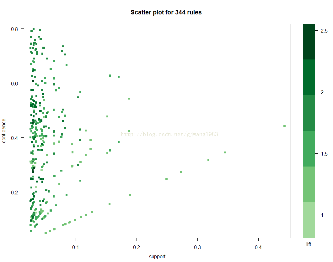
2.1 Scatter Plot

[java] view plain copy

print ?

> plot(second.rules,
+ control=list(jitter=2, col = rev(brewer.pal(9, "Greens")[4:9])),
+ shading = "lift")

shading = "lift"：表示在散点图上颜色深浅的度量是lift。当然也可以设置为support 或者Confidence。

jitter=2：增加抖动值

col: 调色板，默认是100个颜色的灰色调色板。

brewer.pal(n, name): 创建调色板：n表示该调色板内总共有多少种颜色；name表示调色板的名字（参考help）。

这里使用Green这块调色板，引入9中颜色。

这幅散点图表示了规则的分布图：大部分规则的support在0.1以内，Confidence在0-0.8内。每个点的颜色深浅代表了lift的值。

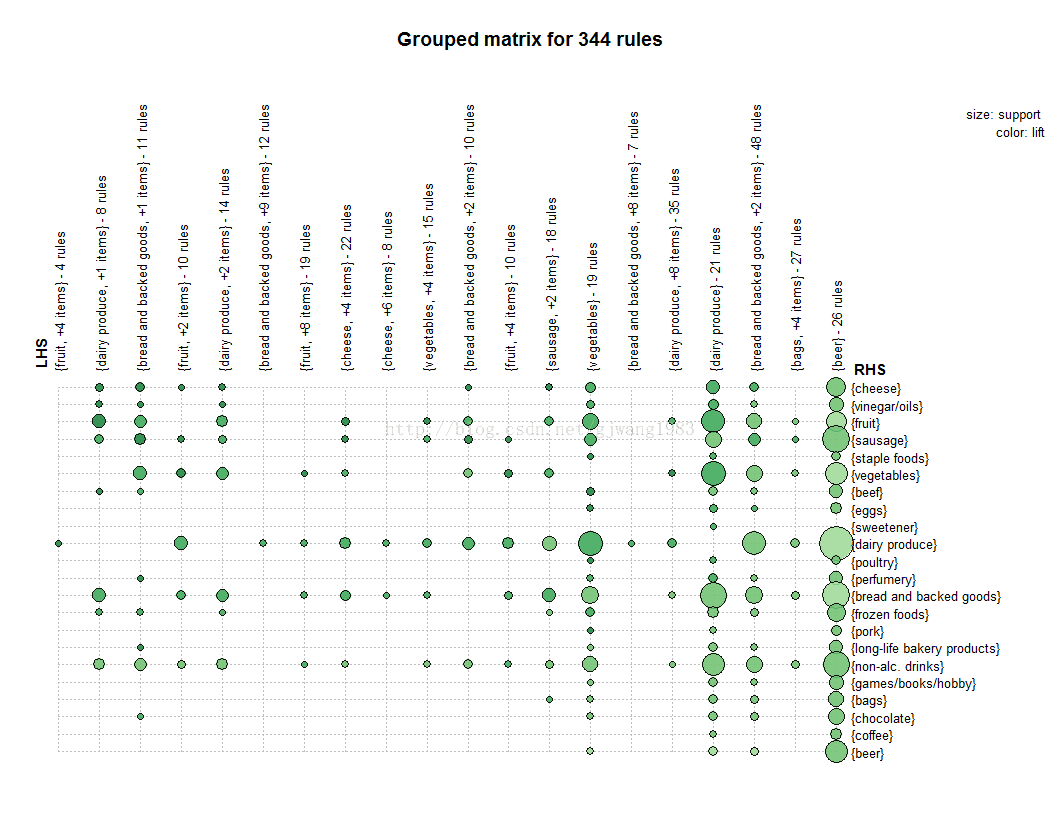
2.2 Grouped Matrix

[java] view plain copy

print ?

> plot(second.rules, method="grouped",
+ control=list(col = rev(brewer.pal(9, "Greens")[4:9])))

Grouped matrix-based visualization.

Antecedents (columns) in the matrix are grouped using clustering. Groups are represented as balloons in the matrix.

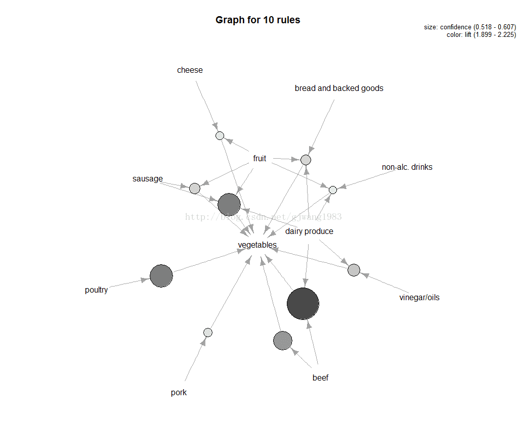
2.3 Graph

Represents the rules (or itemsets) as a graph

[java] view plain copy

print ?

> plot(top.vegie.rules, measure="confidence", method="graph",
+ control=list(type="items"),
+ shading = "lift")

type=items表示每个圆点的入度的item的集合就是LHS的itemset

measure定义了圈圈大小，默认是support

颜色深浅有shading控制

关联规则挖掘小结

1. 关联规则是发现数据间的关系：可能会共同发生的那些属性co-occurrence

2. 一个好的规则可以用lift或者FishersExact Test进行校验。

3. 当属性（商品）越多的时候，支持度会比较低。

4. 关联规则的发掘是交互式的，需要不断的检查、优化。

FP-Growth

TO ADD Here

eclat

arules包中有一个eclat算法的实现，用于发现频繁项集。

例子如下：

[java] view plain copy

print ?

> groceryrules.eclat <- eclat(groceries, parameter = list(support=0.05, minlen=2))
parameter specification:
tidLists support minlen maxlen target ext
FALSE 0.05 2 10 frequent itemsets FALSE
algorithmic control:
sparse sort verbose
7 -2 TRUE
eclat - find frequent item sets with the eclat algorithm
version 2.6 (2004.08.16) (c) 2002-2004 Christian Borgelt
create itemset ...
set transactions ...[169 item(s), 9835 transaction(s)] done [0.01s].
sorting and recoding items ... [28 item(s)] done [0.00s].
creating sparse bit matrix ... [28 row(s), 9835 column(s)] done [0.00s].
writing ... [3 set(s)] done [0.00s].
Creating S4 object ... done [0.00s].
> summary(groceryrules.eclat)
set of 3 itemsets
most frequent items:
whole milk other vegetables rolls/buns yogurt abrasive cleaner (Other)
3 1 1 1 0 0
element (itemset/transaction) length distribution:sizes
2
3
Min. 1st Qu. Median Mean 3rd Qu. Max.
2 2 2 2 2 2
summary of quality measures:
support
Min. :0.05602
1st Qu.:0.05633
Median :0.05663
Mean :0.06250
3rd Qu.:0.06573
Max. :0.07483
includes transaction ID lists: FALSE
mining info:
data ntransactions support
groceries 9835 0.05
> inspect(groceryrules.eclat)
items support
1 {whole milk,
yogurt} 0.05602440
2 {rolls/buns,
whole milk} 0.05663447
3 {other vegetables,
whole milk} 0.07483477