高斯函数（Gaussian function）的详细分析

原文地址：http://blog.csdn.net/jorg_zhao/article/details/52687448

摘要

    论文中遇到很重要的一个元素就是高斯核函数，但是必须要分析出高斯函数的各种潜在属性，本文首先参考相关材料给出高斯核函数的基础，然后使用matlab自动保存不同参数下的高斯核函数的变化gif动图，同时分享出源代码，这样也便于后续的论文写作。

高斯函数的基础

2.1 一维高斯函数

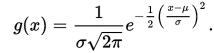
高斯函数，Gaussian Function， 也简称为Gaussian，一维形式如下：

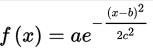
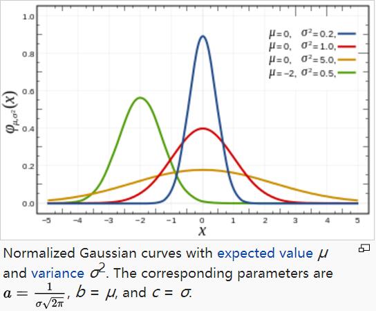
对于任意的实数a,b,c，是以著名数学家Carl Friedrich Gauss的名字命名的。高斯的一维图是特征对称“bell curve”形状，a是曲线尖峰的高度，b是尖峰中心的坐标，c称为标准方差，表征的是bell钟状的宽度。

高斯函数广泛应用于统计学领域，用于表述正态分布，在信号处理领域，用于定义高斯滤波器，在图像处理领域，二维高斯核函数常用于高斯模糊Gaussian Blur，在数学领域，主要是用于解决热力方程和扩散方程，以及定义Weiertrass Transform。

从上图可以看出，高斯函数是一个指数函数，其log函数是对数凹二次函数 whose logarithm a concave quadratic function。

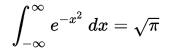
高斯函数的积分是误差函数error function，尽管如此，其在整个实线上的反常积分能够被精确的计算出来，使用如下的高斯积分

同理可得

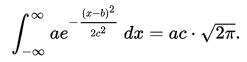
当且仅当

上式积分为1，在这种情况下，高斯是正态分布随机变量的概率密度函数，期望值μ=b，方差delta^2 = c^2，即

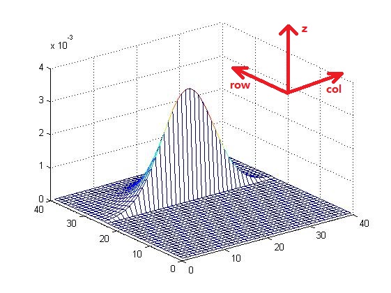
2.2 二维高斯函数

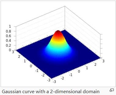
    二维高斯函数，形如

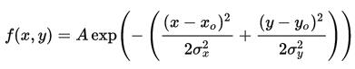
A是幅值，x。y。是中心点坐标，σ_x σ_y是方差，图示如下，A = 1, x_o = 0, y_o = 0, σ_x = σ_y = 1

2.3 高斯函数分析

这一节使用matlab直观的查看高斯函数，在实际编程应用中，高斯函数中的参数有

ksize 高斯函数的大小

sigma 高斯函数的方差

center 高斯函数尖峰中心点坐标

bias 高斯函数尖峰中心点的偏移量，用于控制截断高斯函数

为了方便直观的观察高斯函数参数改变而结果也不一样，下面的代码实现了参数的自动递增，并且将所有的结果图保存为gif图像，首先贴出完整代码：

[plain]  view plain  copy

 print ?

1.  function mainfunc()  
2. % 测试高斯函数，递增的方法实现高斯函数参数的改变对整个高斯函数的影响，  
3. % 并自动保存为gif格式输出。  
4. % created by zhao.buaa 2016.09.28  
5.   
6. %% 保存gif动画  
7. item = 10;      % 迭代次数  
8. dt = 1;             % 步长大小  
9. ksize =20;      % 高斯大小  
10. sigma = 2;      % 方差大小  
11. % filename = ['ksize-' num2str(ksize) '--' num2str(ksize+dt*item) '-sigma-' num2str(sigma) '.gif']; %必须预先建立gif文件  
12. filename = ['ksize-' num2str(ksize)  '-sigma-' num2str(sigma) '--' num2str(sigma+dt*item) '.gif']; %必须预先建立gif文件  
13.   
14. % main loop  
15. for i = 1:item  
16.     center  = round(ksize/2);          % 中心点  
17.     bias       = ksize*10/10;              % 偏移中心点量  
18.     ksigma = ksigma(ksize, sigma, center, bias);    % 构建核函数  
19.     tname  = ['ksize-' num2str(ksize) '-sigma-' num2str(sigma) '-center-' num2str(center)];  
20.     figure(i), mesh(ksigma), title(tname);  
21.     %设置固定的x-y-z坐标范围，便于观察，axis([xmin xmax ymin ymax zmin zmax])  
22.     axis([0 ksize 0 ksize 0 0.008]);  view([0, 90]);% 改变可视角度     
23.     % ksize 递增  
24. %     ksize = ksize + 10;  
25.     % sigma 递增  
26.     sigma = sigma + dt;       
27.       
28.     % 自动保存为gif图像  
29.     frame = getframe(i);  
30.     im = frame2im(frame);  
31.     [I,map] = rgb2ind(im,256);  
32.     if i==1  
33.         imwrite(I,map,filename,'gif','Loopcount',inf, 'DelayTime',0.4);  
34.     else  
35.         imwrite(I,map,filename,'gif','WriteMode','append','DelayTime',0.4);  
36.     end  
37. end;  
38.   
39. close all;  
40.   
41.   
42. %% 截断高斯核函数，截断的程度取决于参数bias  
43. function ksigma = ksigma(ksize, sigma, center,bias)  
44. %ksize = 80;    sigma = 15;  
45. ksigma=fspecial('gaussian',ksize, sigma);   % 构建高斯函数  
46. [m, n] =size(ksigma);  
47. for i = 1:m  
48.     for j = 1:n  
49.         if(  (i<center-bias)||(i>center+bias)||(j<center-bias)||(j>center+bias)  )  
50.             ksigma(i,j) = 0;  
51.         end;  
52.     end;  
53. end;  

结果图：

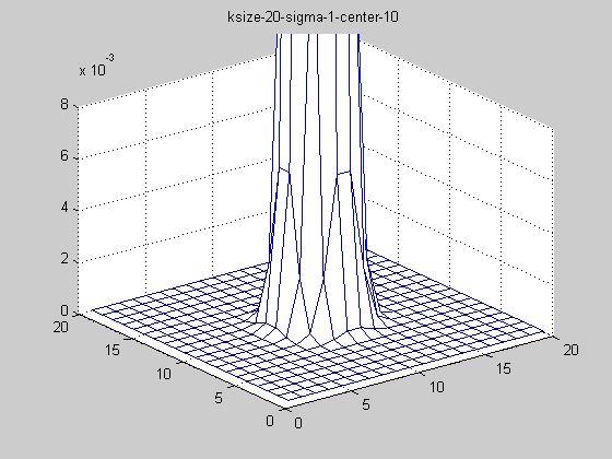
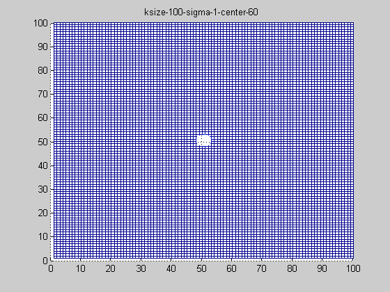
固定ksize为20，sigma从1-9，固定center在高斯中间，并且bias偏移量为整个半径，即原始高斯函数。

随着sigma的增大，整个高斯函数的尖峰逐渐减小，整体也变的更加平缓，则对图像的平滑效果越来越明显。

保持参数不变，对上述高斯函数进行截断，即truncated gaussian function，bias的大小为ksize*3/10，则结果如下图：

truncated gaussian function的作用主要是对超过一定区域的原始图像信息不再考虑，这就保证在更加合理的利用靠近高斯函数中心点的周围像素，同时还可以改变高斯函数的中心坐标，如下图：

为了便于观察截断的效果，改变了可视角度。

高斯核函数卷积

    论文中使用gaussian与feature map做卷积，目前的结果来看，要做到随着到边界的距离改变高斯函数的截断参数，因为图像的边缘如果使用原始高斯函数，就会在边界地方出现特别低的一圈，原因也很简单，高斯函数在与原始图像进行高斯卷积的时候，图像边缘外为0计算的，那么如何解决边缘问题呢？

先看一段代码：

[plain]  view plain  copy

 print ?

1. % 截断高斯核函数  
2. ksize = 40; ksigma=fspecial('gaussian',  ksize, 6);  
3. [m, n] =size(ksigma);  
4. for i = 1:m  
5.     for j = 1:n  
6.         if( i<25 )  
7.            ksigma(i,j) = 0;  
8.         end;  
9.     end;  
10. end;  
11. figure, mesh(ksigma);  

在i，即row上对高斯核函数进行截断，bias为半径大小，则如图6

并且对下图7进行卷积，

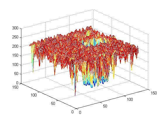
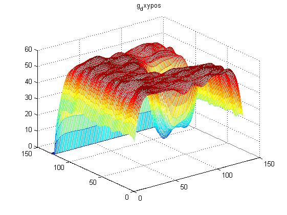
首先卷积核为原始未截断高斯核函数，则结果如图8

可以看出，在图像边缘处的卷积结果出现不想预见的结果，边缘处的值出现大幅度减少的情况，这是高斯核函数在边缘处将图像外的部分当成0计算的结果，因此，需要对高斯核函数进行针对性的截断处理，但是前提是要掌握bias的规律，下面就详细分析。

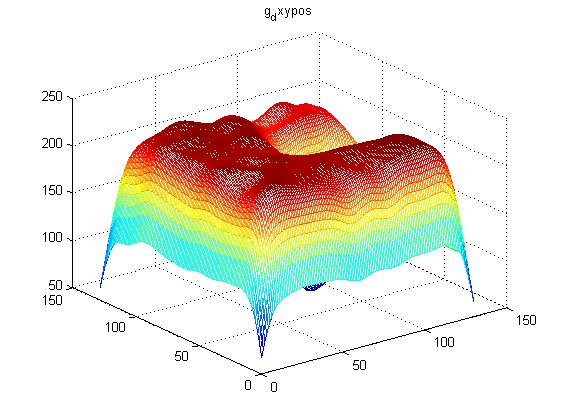
如果使用图6的高斯核函数与图7做卷积操作，则如图9：

可以看出，相比较于图8，与高斯核函数相对应的部分出现了变化，也就是说：

[plain]  view plain  copy

 print ?

1. if( i<25 )  
2.    ksigma(i,j) = 0;  
3. end;  

靠近边缘的时候，改变 i 或 j 的值，即可保证边缘处的平滑处理。但是这样改变高斯核函数，使用matlab不是很好解决这个问题，还是使用将待处理图像边缘向外部扩展bias的大小，与标准高斯核函数做卷积，再将超过原始图像大小的部分剪切掉，目前来看在使用matlab中imfilter函数做卷积运算最合适且最简单的处理方法了，先写在这里，此部分并不是论文中的核心部分，只是数值运算的技巧性编程方法。