


昨天刚参加完一个ibm的医疗影像大赛——我负责的模型是做多目标识别并输出位置的模型。由于之前没有什么经验,采用了在RGB图像上表现不错的Faster-RCNN,但是比赛过程表明:效果不是很好。所以这里把我对Faster-RCNN的原理及代码(https://github.com/yhenon/keras-frcnn)结合起来,分析一下,以厘清Faster-RCNN究竟是什么,它是怎么进行操作的。
一点推荐
作为CSDN的忠实用户,最近发现CSDN学院上了一些对新手比较友好的课程。以我的切身体会来看,对于想要了解机器学习算法或者python编程语言的同学,非常有帮助。还记得我最开始学习python的时候,看的是一本写给小孩子的书(如下)。
虽然这本书不错,但是确实有些过于简单了,而CSDN提供的课程有两门对现在的我来讲还是有相当大的帮助,老师讲课水平高,配合丰富的例子,容易让人掌握知识点,下面推荐两门课程:
人工智能在网络领域的应用与实践:
https://edu.csdn.net/course/play/10319?utm_source=sooner
ps: 如果想要系统学习python的朋友,下面这门课是涵盖了python基础语法、web开发、数据挖掘以及机器学习,是CSDN强力推荐的课程,有需要的朋友可以看看哈:
Python全栈工程师:
https://edu.csdn.net/topic/python115?utm_source=sooner
① 简单介绍
Faster RCNN可以看做**“区域生成网络(RPN)+Fast RCNN“的系统,用RPN代替Fast RCNN中的Selective Search来进行候选框的选择和修正。
Faster RCNN是由Ross Girshick于2015年提出的,其团队的何凯明大神(Resnet的发明者)将这个新的方法用于实时的目标检测**(Real-Time Object Detection),简单网络目标检测速度达到17fps,在PASCAL VOC上准确率为59.9%;复杂网络达到5fps,准确率78.8%。
② RPN+Fast RCNN的思路
从RCNN到Fast RCNN,再到这里的Faster RCNN,目标检测的四个基本步骤(候选区域生成,特征提取,目标分类,位置回归修正)终于被统一到一个深度网络框架之内。所有计算没有重复,完全在GPU中完成,从而显著的提高了运行速度。
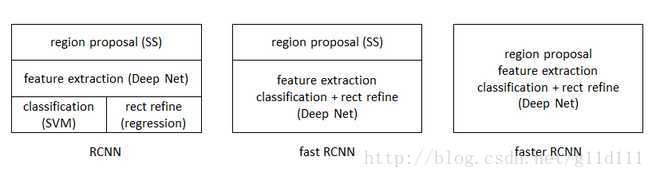
此图来自shenxiaolu1984的博客,在此感谢一下。
Faster-RCNN的做法是:
• 将RPN放在最后一个卷积层的后面
• RPN直接训练得到候选区域
本系列文章:
将结合代码(Python-keras)详细的介绍Faster-RCNN及其相关内容,并补充一些有用的技巧。
③ Faster-RCN的结构
在这里,基本的思路是:在经过比较常用的用于ImageNet分类(如VGG,Resnet等)上提取好的特征图上,对所有可能的**候选框(Bounding box)**进行判别。后续对Bbox还有回归来修正坐标的步骤,所以候选框实际上是比较稀疏的。
其步骤如下:
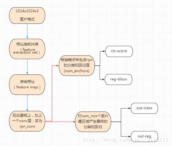
④ 特征提取(提出feature map)
原始特征提取(上图第二步)包含若干层conv+maxpooling,直接套用ImageNet上常见的分类网络即可。这里以VGG为例,其结构形式为:
# coding: UTF-8
from keras.layers import Flatten, Dense, Input, Conv2D, MaxPooling2D, Dropout
from keras.layers import GlobalAveragePooling2D, GlobalMaxPooling2D, TimeDistributed

# 注意: theano和tensorflow作为后端的时候,接收图片格式不一致。
if K.image_dim_ordering() == 'th':
	# theano 接收形式为channel, width, height
	input_shape_img = (3, None, None)
else:
	# tensorflow 接收形式为width, height, channel
	input_shape_img = (None, None, 3)
img_input = Input(shape=input_shape_img)

def nn_base(img_input):
	# Block 1
    x = Conv2D(64, (3, 3), activation='relu', padding='same', name='block1_conv1')(img_input)
    x = Conv2D(64, (3, 3), activation='relu', padding='same', name='block1_conv2')(x)
    # 缩水1/2 1024x1024 -> 512x512
    x = MaxPooling2D((2, 2), strides=(2, 2), name='block1_pool')(x)

    # Block 2
    x = Conv2D(128, (3, 3), activation='relu', padding='same', name='block2_conv1')(x)
    x = Conv2D(128, (3, 3), activation='relu', padding='same', name='block2_conv2')(x)
    # 缩水1/2 512x512 -> 256x256
    x = MaxPooling2D((2, 2), strides=(2, 2), name='block2_pool')(x)

    # Block 3
    x = Conv2D(256, (3, 3), activation='relu', padding='same', name='block3_conv1')(x)
    x = Conv2D(256, (3, 3), activation='relu', padding='same', name='block3_conv2')(x)
    x = Conv2D(256, (3, 3), activation='relu', padding='same', name='block3_conv3')(x)
    # 缩水1/2 256x256 -> 128x128
    x = MaxPooling2D((2, 2), strides=(2, 2), name='block3_pool')(x)

    # Block 4
    x = Conv2D(512, (3, 3), activation='relu', padding='same', name='block4_conv1')(x)
    x = Conv2D(512, (3, 3), activation='relu', padding='same', name='block4_conv2')(x)
    x = Conv2D(512, (3, 3), activation='relu', padding='same', name='block4_conv3')(x)
    # 缩水1/2 128x128 -> 64x64
    x = MaxPooling2D((2, 2), strides=(2, 2), name='block4_pool')(x)

    # Block 5
    x = Conv2D(512, (3, 3), activation='relu', padding='same', name='block5_conv1')(x)
    x = Conv2D(512, (3, 3), activation='relu', padding='same', name='block5_conv2')(x)
    x = Conv2D(512, (3, 3), activation='relu', padding='same', name='block5_conv3')(x)

    # 显然,最后返回的x是64x64x512的feature map。
    return x
以这个nn_base函数的返回值x作为后续的base_layers,紧接着,在base_layers后面添加一个conv层,并作为rpn的回归和分类的输入:
# 这里num_anchors = 3x3 = 9,后面会提到
def rpn(base_layers, num_anchors):

    x = Conv2D(512, (3, 3), padding='same', activation='relu', kernel_initializer='normal', name='rpn_conv1')(base_layers)

    # rpn分类和回归
    x_class = Conv2D(num_anchors, (1, 1), activation='sigmoid', kernel_initializer='uniform', name='rpn_out_class')(x)
    x_reg = Conv2D(num_anchors * 4, (1, 1), activation='linear', kernel_initializer='zero', name='rpn_out_regress')(x)

    return [x_class, x_reg, base_layers]
这里,x_class是使用11的卷积核在rpn_conv1上进行卷积,生成了num_anchors数量的channel ,每个channel包含特征图(wh)个sigmoid激活值,表明该anchor是否可用,与我们刚刚计算的y_rpn_cls对应。同样地,x_regr与刚刚计算的y_rpn_regr对应。
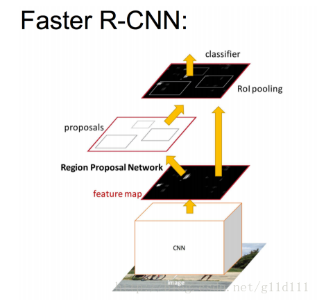
⑤ RPN(Region Proposal Networks)的设计和训练思路
如下图所示,RPN是在CNN训练得到的用于分类任务的feature map基础上,进行
• 在feature map上滑动窗口。
• 建一个神经网络用于物体分类(x_class)+框位置的回归(x_reg)。
• 滑动窗口的位置提供了物体的大体位置信息。
• 框的回归修正框的位置,使其与对应的bbox位置更相近。
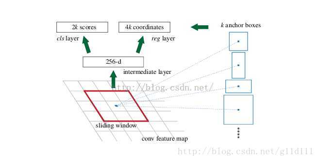
SPP的映射机制
上图是RPN的网络流程图,即利用了SPP的映射机制,从上面的rpn_conv1上进行滑窗来替代从原图滑窗。
不过,要如何训练出一个网络来替代selective search相类似的功能呢?
实际上思路很简单,就是先通过SPP根据一一对应的点从rpn_conv1映射回原图,根据设计不同的固定初始尺度训练一个网络,就是给它大小不同(但设计固定)的region图,然后根据与ground truth的覆盖率给它正负标签,让它学习里面是否有object即可。
这就又变成介绍RCNN之前提出的traditional method,训练出一个能检测物体的网络,然后对整张图片进行滑窗判断,不过这样子的话由于无法判断region的尺度和scale ratio,故需要多次放缩,这样子测试,估计判断一张图片是否有物体就需要很久。(传统hog+svm->dpm)
如何降低这一部分的复杂度?
要知道我们只需要找出大致的地方,无论是精确定位位置还是尺寸,后面的工作都可以完成。鉴于此,用层数低的网络还不如用深层的网络,通过① 固定anchor_box_scales变化,②固定anchor_box_ratios变化,③固定的采样方式(反正后面的工作能进行调整,更何况它本身就可以对box的位置进行调整)这样子来降低任务复杂度呢。
这里有个很不错的地方就是在前面可以共享卷积计算结果(第四部分的base_layers),这也算是用深度网络的另一个原因吧。
文章叫这些proposal region为anchor(锚点)的原因也正是这三个固定的变化。这个网络的结果就是卷积层的每个点都有有关于k个achor boxes的输出,包括是不是物体,调整box相应的位置。这相当于给了比较死的初始位置(三个固定),然后来大致判断是否是物体以及所对应的位置.
这样子的话RPN所要做的也就完成了,这个网络也就完成了它应该完成的使命,剩下的交给其他部分完成。
⑥ 锚点位置(anchor)
特征可以看做一个尺度64x64x512的特征图(feature map),对于该图像的每一个位置,考虑9个可能的候选窗口(即前面的num_anchors):三种面积[128,256,512] × 三种比例[1:1,1:2,2:1] 。
这九种可能的窗口形式分别为:
| Window | Scale | Ratio |
|---|---|---|
| 128 x 128 | 128 | 1:1 |
| 128 x 256 | 128 | 1:2 |
| 128 x 64 | 128 | 2:1 |
| 256 x 256 | 256 | 1:1 |
| 256 x 512 | 256 | 1:2 |
| 256 x 128 | 256 | 2:1 |
| 512 x 512 | 512 | 1:1 |
| 512 x 1024 | 512 | 1:2 |
| 512 x 256 | 512 | 2:1 |
这些候选窗口称为anchors。
注意:这里采用一个Config类来表示Faster-RCNN对应的各种参数(包括上面说的面积和比例关系等)
from keras import backend as K
import math

class Config:

	def __init__(self):

		self.verbose = True

		self.network = 'vgg'

		# setting for data augmentation
		self.use_horizontal_flips = False
		self.use_vertical_flips = False
		self.rot_90 = False


		# 比赛的时候,调整anchor_box_scales和anchor_box_ratios
		# anchor box scales
		self.anchor_box_scales = [128, 256, 512]

		# anchor box ratios
		self.anchor_box_ratios = [[1, 1], [1./math.sqrt(2), 2./math.sqrt(2)], [2./math.sqrt(2), 1./math.sqrt(2)]]

		# size to resize the smallest side of the image
		self.im_size = 600

		# image channel-wise mean to subtract
		self.img_channel_mean = [103.939, 116.779, 123.68]
		self.img_scaling_factor = 1.0

		# number of ROIs at once
		self.num_rois = 4

		# stride at the RPN (this depends on the network configuration)
		self.rpn_stride = 16

		self.balanced_classes = False

		# scaling the stdev
		# 基于样本估算标准偏差。标准偏差反映数值相对于平均值(mean) 的离散程度。
		self.std_scaling = 4.0
		self.classifier_regr_std = [8.0, 8.0, 4.0, 4.0]

		# overlaps for RPN
		self.rpn_min_overlap = 0.3
		self.rpn_max_overlap = 0.7

		# overlaps for classifier ROIs
		self.classifier_min_overlap = 0.3
		self.classifier_max_overlap = 0.8

		# placeholder for the class mapping, automatically generated by the parser
		self.class_mapping = None

		#location of pretrained weights for the base network
		# weight files can be found at:
		# https://github.com/fchollet/deep-learning-models/releases/download/v0.2/resnet50_weights_th_dim_ordering_th_kernels_notop.h5
		# https://github.com/fchollet/deep-learning-models/releases/download/v0.2/resnet50_weights_tf_dim_ordering_tf_kernels_notop.h5

		self.model_path = 'model_frcnn.vgg.hdf5'
从下面的calc_rpn函数可以看出,有四层循环:1、2层为取出框的尺寸大小。3、4层为选定锚点的坐标,并与实际经过缩放对应的bbox的坐标(x1,y1表示矩形框左上角,x2, y2表示右下角)计算IoU以及进行判断每个锚点对应的9种框是否能匹配到bbox,以及匹配的程度。
# coding: UTF-8
from __future__ import absolute_import
import numpy as np
import cv2
import random
import copy
# 这里C代表一个参数类(上面的Config),C = Config()
def calc_rpn(C, img_data, width, height, resized_width, resized_height, img_length_calc_function):


	# 接下来读取了几个参数,downscale就是从图片到特征图的缩放倍数(默认为16.0) 这里,
	# img_length_calc_function(也就是实际的vgg中的get_img_output_length中整除的值一样。)
	# anchor_size和anchor_ratios是我们初步选区大小的参数,比如3个size和3个ratios,可以组合成9种不同形状大小的选区。
	downscale = float(C.rpn_stride)
	anchor_sizes = C.anchor_box_scales
	anchor_ratios = C.anchor_box_ratios
	num_anchors = len(anchor_sizes) * len(anchor_ratios)

	# calculate the output map size based on the network architecture
	# 接下来,
	# 通过img_length_calc_function 对VGG16 返回的是一个height和width都整除16的结果这个方法计算出了特征图的尺寸。
	# output_width = output_height = 600 // 16 = 37
	(output_width, output_height) = img_length_calc_function(resized_width, resized_height)


	# 下一步是几个变量初始化可以先不看,后面用到的时候再看。

	# n_anchratios = 3
	n_anchratios = len(anchor_ratios)

	# initialise empty output objectives
	y_rpn_overlap = np.zeros((output_height, output_width, num_anchors))
	y_is_box_valid = np.zeros((output_height, output_width, num_anchors))
	y_rpn_regr = np.zeros((output_height, output_width, num_anchors * 4))

	num_bboxes = len(img_data['bboxes'])

	num_anchors_for_bbox = np.zeros(num_bboxes).astype(int)
	best_anchor_for_bbox = -1*np.ones((num_bboxes, 4)).astype(int)
	best_iou_for_bbox = np.zeros(num_bboxes).astype(np.float32)
	best_x_for_bbox = np.zeros((num_bboxes, 4)).astype(int)
	best_dx_for_bbox = np.zeros((num_bboxes, 4)).astype(np.float32)


	# 因为我们的计算都是基于resize以后的图像的,所以接下来把bbox中的x1,x2,y1,y2分别通过缩放匹配到resize以后的图像。
	# 这里记做gta,尺寸为(num_of_bbox,4)。
	# get the GT box coordinates, and resize to account for image resizing
	gta = np.zeros((num_bboxes, 4))
	for bbox_num, bbox in enumerate(img_data['bboxes']):
		# get the GT box coordinates, and resize to account for image resizing
		gta[bbox_num, 0] = bbox['x1'] * (resized_width / float(width))
		gta[bbox_num, 1] = bbox['x2'] * (resized_width / float(width))
		gta[bbox_num, 2] = bbox['y1'] * (resized_height / float(height))
		gta[bbox_num, 3] = bbox['y2'] * (resized_height / float(height))

	# rpn ground truth
	# 这一段计算了anchor的长宽,然后比较重要的就是把特征图的每一个点作为一个锚点,
	# 通过乘以downscale,映射到图片的实际尺寸,再结合anchor的尺寸,忽略掉超出图片范围的。
	# 一个个大小、比例不一的矩形选框就跃然纸上了。
	# 第一层for 3层
	# 第二层for 3层
	for anchor_size_idx in range(len(anchor_sizes)):
		for anchor_ratio_idx in range(n_anchratios):
			# 框的尺寸选定
			anchor_x = anchor_sizes[anchor_size_idx] * anchor_ratios[anchor_ratio_idx][0]
			anchor_y = anchor_sizes[anchor_size_idx] * anchor_ratios[anchor_ratio_idx][1]
			# 对1024 --> 600 --> 37的形式,output_width = 37
			# 选定锚点坐标: x_anc y_anc
			for ix in range(output_width):
				# x-coordinates of the current anchor box
				x1_anc = downscale * (ix + 0.5) - anchor_x / 2
				x2_anc = downscale * (ix + 0.5) + anchor_x / 2

				# ignore boxes that go across image boundaries
				if x1_anc < 0 or x2_anc > resized_width:
					continue

				for jy in range(output_height):

					# y-coordinates of the current anchor box
					y1_anc = downscale * (jy + 0.5) - anchor_y / 2
					y2_anc = downscale * (jy + 0.5) + anchor_y / 2

					# ignore boxes that go across image boundaries
					if y1_anc < 0 or y2_anc > resized_height:
						continue


					# 定义了两个变量,bbox_type和best_iou_for_loc,后面会用到。计算了anchor与gta的交集 iou(),
					# 然后就是如果交集大于best_iou_for_bbox[bbox_num]或者大于我们设定的阈值,就会去计算gta和anchor的中心点坐标,
					# bbox_type indicates whether an anchor should be a target
					bbox_type = 'neg'

					# this is the best IOU for the (x,y) coord and the current anchor
					# note that this is different from the best IOU for a GT bbox
					best_iou_for_loc = 0.0

					# 对选出的选择框,判断其和实际上图片的所有Bbox中,有无满足大于规定threshold的情况。
					for bbox_num in range(num_bboxes):

						# get IOU of the current GT box and the current anchor box
						curr_iou = iou([gta[bbox_num, 0], gta[bbox_num, 2], gta[bbox_num, 1], gta[bbox_num, 3]], [x1_anc, y1_anc, x2_anc, y2_anc])
						# calculate the regression targets if they will be needed
						# 默认的最大rpn重叠部分(rpn_max_overlap)为0.7,最小(rpn_min_overlap)为0.3
						if curr_iou > best_iou_for_bbox[bbox_num] or curr_iou > C.rpn_max_overlap:
							cx = (gta[bbox_num, 0] + gta[bbox_num, 1]) / 2.0
							cy = (gta[bbox_num, 2] + gta[bbox_num, 3]) / 2.0
							cxa = (x1_anc + x2_anc)/2.0
							cya = (y1_anc + y2_anc)/2.0

							# 计算出x,y,w,h四个值的梯度值。
							# 为什么要计算这个梯度呢?因为RPN计算出来的区域不一定是很准确的,从只有9个尺寸的anchor也可以推测出来,
							# 因此我们在预测时还会进行一次回归计算,而不是直接使用这个区域的坐标。
							tx = (cx - cxa) / (x2_anc - x1_anc)
							ty = (cy - cya) / (y2_anc - y1_anc)
							tw = np.log((gta[bbox_num, 1] - gta[bbox_num, 0]) / (x2_anc - x1_anc))
							th = np.log((gta[bbox_num, 3] - gta[bbox_num, 2]) / (y2_anc - y1_anc))

						# 前提是:当前的bbox不是背景 != 'bg'
						if img_data['bboxes'][bbox_num]['class'] != 'bg':

							# all GT boxes should be mapped to an anchor box, so we keep track of which anchor box was best
							if curr_iou > best_iou_for_bbox[bbox_num]:
								# jy 高度 ix 宽度
								best_anchor_for_bbox[bbox_num] = [jy, ix, anchor_ratio_idx, anchor_size_idx]
								best_iou_for_bbox[bbox_num] = curr_iou
								best_x_for_bbox[bbox_num,:] = [x1_anc, x2_anc, y1_anc, y2_anc]
								best_dx_for_bbox[bbox_num,:] = [tx, ty, tw, th]

							# we set the anchor to positive if the IOU is >0.7 (it does not matter if there was another better box, it just indicates overlap)
							if curr_iou > C.rpn_max_overlap:
								bbox_type = 'pos'
								# 因为num_anchors_for_bbox 形式为 [0, 0, 0, 0]
								# 这步操作的结果为 [1, 1, 1, 1]
								num_anchors_for_bbox[bbox_num] += 1
								# we update the regression layer target if this IOU is the best for the current (x,y) and anchor position
								if curr_iou > best_iou_for_loc:
									# 不断修正最佳iou对应的区域和梯度
									best_iou_for_loc = curr_iou
									best_grad = (tx, ty, tw, th)

							# if the IOU is >0.3 and <0.7, it is ambiguous and no included in the objective
							if C.rpn_min_overlap < curr_iou < C.rpn_max_overlap:
								# gray zone between neg and pos
								if bbox_type != 'pos':
									bbox_type = 'neutral'

					# turn on or off outputs depending on IOUs
					# 接下来根据bbox_type对本anchor进行打标,y_is_box_valid和y_rpn_overlap分别定义了这个anchor是否可用和是否包含对象。
					if bbox_type == 'neg':
						y_is_box_valid[jy, ix, anchor_ratio_idx + n_anchratios * anchor_size_idx] = 1
						y_rpn_overlap[jy, ix, anchor_ratio_idx + n_anchratios * anchor_size_idx] = 0
					elif bbox_type == 'neutral':
						y_is_box_valid[jy, ix, anchor_ratio_idx + n_anchratios * anchor_size_idx] = 0
						y_rpn_overlap[jy, ix, anchor_ratio_idx + n_anchratios * anchor_size_idx] = 0
					elif bbox_type == 'pos':
						y_is_box_valid[jy, ix, anchor_ratio_idx + n_anchratios * anchor_size_idx] = 1
						y_rpn_overlap[jy, ix, anchor_ratio_idx + n_anchratios * anchor_size_idx] = 1
						# 默认是36个选择
						start = 4 * (anchor_ratio_idx + n_anchratios * anchor_size_idx)
						y_rpn_regr[jy, ix, start:start+4] = best_grad


	# we ensure that every bbox has at least one positive RPN region
	# 这里又出现了一个潜在问题: 可能会有bbox可能找不到心仪的anchor,那这些训练数据就没法利用了,
	# 因此我们用一个折中的办法来保证每个bbox至少有一个anchor与之对应。
	# 下面是具体的方法,比较简单,对于没有对应anchor的bbox,在中性anchor里挑最好的,当然前提是你不能跟我完全不相交,那就太过分了。。
	for idx in range(num_anchors_for_bbox.shape[0]):
		if num_anchors_for_bbox[idx] == 0:
			# no box with an IOU greater than zero ... 遇到这种情况只能pass了
			if best_anchor_for_bbox[idx, 0] == -1:
				continue
			y_is_box_valid[
				best_anchor_for_bbox[idx,0], best_anchor_for_bbox[idx,1], best_anchor_for_bbox[idx,2] + n_anchratios *
				best_anchor_for_bbox[idx,3]] = 1
			y_rpn_overlap[
				best_anchor_for_bbox[idx,0], best_anchor_for_bbox[idx,1], best_anchor_for_bbox[idx,2] + n_anchratios *
				best_anchor_for_bbox[idx,3]] = 1
			start = 4 * (best_anchor_for_bbox[idx,2] + n_anchratios * best_anchor_for_bbox[idx,3])
			y_rpn_regr[
				best_anchor_for_bbox[idx,0], best_anchor_for_bbox[idx,1], start:start+4] = best_dx_for_bbox[idx, :]

	# y_rpn_overlap 原来的形式np.zeros((output_height, output_width, num_anchors))
	# 现在变为 (num_anchors, output_height, output_width)
	y_rpn_overlap = np.transpose(y_rpn_overlap, (2, 0, 1))
    # (新的一列,num_anchors, output_height, output_width)
	y_rpn_overlap = np.expand_dims(y_rpn_overlap, axis=0)

	y_is_box_valid = np.transpose(y_is_box_valid, (2, 0, 1))
	y_is_box_valid = np.expand_dims(y_is_box_valid, axis=0)

	y_rpn_regr = np.transpose(y_rpn_regr, (2, 0, 1))
	y_rpn_regr = np.expand_dims(y_rpn_regr, axis=0)

    # pos表示box neg表示背景
	pos_locs = np.where(np.logical_and(y_rpn_overlap[0, :, :, :] == 1, y_is_box_valid[0, :, :, :] == 1))
	neg_locs = np.where(np.logical_and(y_rpn_overlap[0, :, :, :] == 0, y_is_box_valid[0, :, :, :] == 1))

	num_pos = len(pos_locs[0])

	# one issue is that the RPN has many more negative than positive regions, so we turn off some of the negative
	# regions. We also limit it to 256 regions.
    # 因为negtive的anchor肯定远多于postive的,
    # 因此在这里设定了regions数量的最大值为256,并对pos和neg的样本进行了均匀的取样。
	num_regions = 256

    # 对感兴趣的框超过128的时候...
	if len(pos_locs[0]) > num_regions/2:
        # val_locs为一个list
		val_locs = random.sample(range(len(pos_locs[0])), len(pos_locs[0]) - num_regions/2)
		y_is_box_valid[0, pos_locs[0][val_locs], pos_locs[1][val_locs], pos_locs[2][val_locs]] = 0
		num_pos = num_regions/2
    # 使得neg(背景)和pos(锚框)数量一致
	if len(neg_locs[0]) + num_pos > num_regions:
		val_locs = random.sample(range(len(neg_locs[0])), len(neg_locs[0]) - num_pos)
		y_is_box_valid[0, neg_locs[0][val_locs], neg_locs[1][val_locs], neg_locs[2][val_locs]] = 0
    # axis = 1按行拼接
    # a = [[1 2 3]
    # [4 5 6]]
    # b = [[11 21 31]
    #  [ 7  8  9]]
    # np.concatenate((a,b), axis=1) =
    # [[ 1  2  3 11 21 31]
    #  [ 4  5  6  7  8  9]]

	y_rpn_cls = np.concatenate([y_is_box_valid, y_rpn_overlap], axis=1)
	y_rpn_regr = np.concatenate([np.repeat(y_rpn_overlap, 4, axis=1), y_rpn_regr], axis=1)
    # 最后,得到了两个返回值y_rpn_cls,y_rpn_regr。分别用于确定anchor是否包含物体,和回归梯度。
    # 值得注意的是, y_rpn_cls和y_rpn_regr数量是比实际的输入图片对应的Bbox数量多挺多的。
	return np.copy(y_rpn_cls), np.copy(y_rpn_regr)
这里简单介绍一下IoU,可以理解将IoU简单理解为是一个定位精度评价公式。IoU定义了两个bounding box的重叠度,如下图所示:
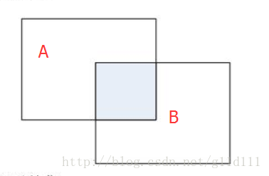
其中蓝色部分为A和B的交集:
A
∩
B
A ∩ B
A∩B
那么矩形框A、B的一个重合度IOU计算公式为:
I
O
U
=
(
A
∩
B
)
/
(
A
∪
B
)
IOU=(A∩B)/(A∪B)
IOU=(A∩B)/(A∪B)
对应的函数为:
# 重合度
def iou(a, b):
	# a and b should be (x1,y1,x2,y2)

	if a[0] >= a[2] or a[1] >= a[3] or b[0] >= b[2] or b[1] >= b[3]:
		return 0.0
	# 注意,intersection 和 union 需要自定义,这个比较简单,此处略过
	area_i = intersection(a, b) # 交集
	area_u = union(a, b, area_i) # 并集

	return float(area_i) / float(area_u + 1e-6)
小结
在整个Faster RCNN算法中,有三种尺度。
-
原图尺度:原始输入的大小。不受任何限制,不影响性能。
-
归一化尺度:输入特征提取网络的大小,在测试时设置,上面的Config类中size to resize the smallest side of the image,self.im_size = 600。anchor在这个尺度上设定。这个参数和anchor的相对大小决定了想要检测的目标范围。
-
网络输入尺度:输入特征检测网络的大小,在训练时设置。
参考资料
[1] RCNN学习笔记(5):faster rcnn
[2] Fast RCNN算法详解
[3] 深度学习(十八)基于R-CNN的物体检测


 205
205


 被折叠的 条评论
为什么被折叠?
被折叠的 条评论
为什么被折叠?
 到【灌水乐园】发言


