Softmax算法：逻辑回归的扩展

最新推荐文章于 2023-12-11 23:06:39 发布

haoji007

最新推荐文章于 2023-12-11 23:06:39 发布

阅读量812

点赞数

分类专栏：【 ML优化方法】

【 ML优化方法】专栏收录该内容

18 篇文章 2 订阅

订阅专栏

Softmax回归

[hide]

简介

在本节中，我们介绍Softmax回归模型，该模型是logistic回归模型在多分类问题上的推广，在多分类问题中，类标签 $\textstyle y$ 可以取两个以上的值。 Softmax回归模型对于诸如MNIST手写数字分类等问题是很有用的，该问题的目的是辨识10个不同的单个数字。Softmax回归是有监督的，不过后面也会介绍它与深度学习/无监督学习方法的结合。（译者注： MNIST 是一个手写数字识别库，由NYU 的Yann LeCun 等人维护。http://yann.lecun.com/exdb/mnist/ ）

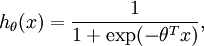
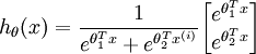
回想一下在 logistic 回归中，我们的训练集由 $\textstyle m$ 个已标记的样本构成： $\{ (x^{(1)}, y^{(1)}), \ldots, (x^{(m)}, y^{(m)}) \}$ ，其中输入特征 $x^{(i)} \in \Re^{n+1}$ 。（我们对符号的约定如下：特征向量 $\textstyle x$ 的维度为 $\textstyle n+1$ ，其中 $\textstyle x_0 = 1$ 对应截距项。）由于 logistic 回归是针对二分类问题的，因此类标记 $y^{(i)} \in \{0,1\}$ 。假设函数(hypothesis function) 如下：

$\begin{align}h_\theta(x) = \frac{1}{1+\exp(-\theta^Tx)},\end{align}$

我们将训练模型参数 $\textstyle \theta$ ，使其能够最小化代价函数：

$\begin{align}J(\theta) = -\frac{1}{m} \left[ \sum_{i=1}^m y^{(i)} \log h_\theta(x^{(i)}) + (1-y^{(i)}) \log (1-h_\theta(x^{(i)})) \right]\end{align}$

在 softmax回归中，我们解决的是多分类问题（相对于 logistic 回归解决的二分类问题），类标 $\textstyle y$ 可以取 $\textstyle k$ 个不同的值（而不是 2 个）。因此，对于训练集 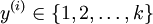$\{ (x^{(1)}, y^{(1)}), \ldots, (x^{(m)}, y^{(m)}) \}$ ，我们有 $y^{(i)} \in \{1, 2, \ldots, k\}$ 。（注意此处的类别下标从 1 开始，而不是 0）。例如，在 MNIST 数字识别任务中，我们有 $\textstyle k=10$ 个不同的类别。

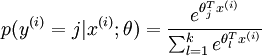
对于给定的测试输入 $\textstyle x$ ，我们想用假设函数针对每一个类别j估算出概率值 $\textstyle p(y=j | x)$ 。也就是说，我们想估计 $\textstyle x$ 的每一种分类结果出现的概率。因此，我们的假设函数将要输出一个 $\textstyle k$ 维的向量（向量元素的和为1）来表示这 $\textstyle k$ 个估计的概率值。具体地说，我们的假设函数 $\textstyle h_{\theta}(x)$ 形式如下：

$\begin{align}h_\theta(x^{(i)}) =\begin{bmatrix}p(y^{(i)} = 1 | x^{(i)}; \theta) \\p(y^{(i)} = 2 | x^{(i)}; \theta) \\\vdots \\p(y^{(i)} = k | x^{(i)}; \theta)\end{bmatrix}=\frac{1}{ \sum_{j=1}^{k}{e^{ \theta_j^T x^{(i)} }} }\begin{bmatrix}e^{ \theta_1^T x^{(i)} } \\e^{ \theta_2^T x^{(i)} } \\\vdots \\e^{ \theta_k^T x^{(i)} } \\\end{bmatrix}\end{align}$

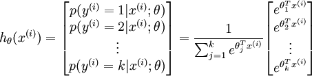
其中 $\theta_1, \theta_2, \ldots, \theta_k \in \Re^{n+1}$ 是模型的参数。请注意 $\frac{1}{ \sum_{j=1}^{k}{e^{ \theta_j^T x^{(i)} }} }$ 这一项对概率分布进行归一化，使得所有概率之和为 1 。

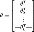
为了方便起见，我们同样使用符号 $\textstyle \theta$ 来表示全部的模型参数。在实现Softmax回归时，将 $\textstyle \theta$ 用一个 $\textstyle k \times(n+1)$ 的矩阵来表示会很方便，该矩阵是将 $\theta_1, \theta_2, \ldots, \theta_k$ 按行罗列起来得到的，如下所示：

$\theta = \begin{bmatrix}\mbox{---} \theta_1^T \mbox{---} \\\mbox{---} \theta_2^T \mbox{---} \\\vdots \\\mbox{---} \theta_k^T \mbox{---} \\\end{bmatrix}$

代价函数

现在我们来介绍 softmax 回归算法的代价函数。在下面的公式中， $\textstyle 1\{\cdot\}$ 是示性函数，其取值规则为：

 值为真的表达式

， $\textstyle 1\{$ 值为假的表达式 $\textstyle \}=0$ 。举例来说，表达式 $\textstyle 1\{2+2=4\}$ 的值为1 ， $\textstyle 1\{1+1=5\}$ 的值为 0。我们的代价函数为：

$\begin{align}J(\theta) = - \frac{1}{m} \left[ \sum_{i=1}^{m} \sum_{j=1}^{k} 1\left\{y^{(i)} = j\right\} \log \frac{e^{\theta_j^T x^{(i)}}}{\sum_{l=1}^k e^{ \theta_l^T x^{(i)} }}\right]\end{align}$

值得注意的是，上述公式是logistic回归代价函数的推广。logistic回归代价函数可以改为：

$\begin{align}J(\theta) &= -\frac{1}{m} \left[ \sum_{i=1}^m (1-y^{(i)}) \log (1-h_\theta(x^{(i)})) + y^{(i)} \log h_\theta(x^{(i)}) \right] \\&= - \frac{1}{m} \left[ \sum_{i=1}^{m} \sum_{j=0}^{1} 1\left\{y^{(i)} = j\right\} \log p(y^{(i)} = j | x^{(i)} ; \theta) \right]\end{align}$

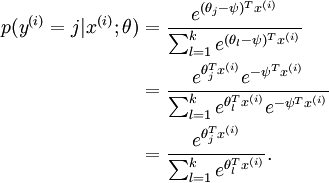
可以看到，Softmax代价函数与logistic 代价函数在形式上非常类似，只是在Softmax损失函数中对类标记的 $\textstyle k$ 个可能值进行了累加。注意在Softmax回归中将 $\textstyle x$ 分类为类别 $\textstyle j$ 的概率为：

$p(y^{(i)} = j | x^{(i)} ; \theta) = \frac{e^{\theta_j^T x^{(i)}}}{\sum_{l=1}^k e^{ \theta_l^T x^{(i)}} }$ .

对于 $\textstyle J(\theta)$ 的最小化问题，目前还没有闭式解法。因此，我们使用迭代的优化算法（例如梯度下降法，或 L-BFGS）。经过求导，我们得到梯度公式如下：

$\begin{align}\nabla_{\theta_j} J(\theta) = - \frac{1}{m} \sum_{i=1}^{m}{ \left[ x^{(i)} \left( 1\{ y^{(i)} = j\} - p(y^{(i)} = j | x^{(i)}; \theta) \right) \right] }\end{align}$

让我们来回顾一下符号 " $\textstyle \nabla_{\theta_j}$ " 的含义。 $\textstyle \nabla_{\theta_j} J(\theta)$ 本身是一个向量，它的第 $\textstyle l$ 个元素 $\textstyle \frac{\partial J(\theta)}{\partial \theta_{jl}}$ 是 $\textstyle J(\theta)$ 对 $\textstyle \theta_j$ 的第 $\textstyle l$ 个分量的偏导数。

有了上面的偏导数公式以后，我们就可以将它代入到梯度下降法等算法中，来最小化 $\textstyle J(\theta)$ 。例如，在梯度下降法的标准实现中，每一次迭代需要进行如下更新: 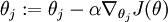$\textstyle \theta_j := \theta_j - \alpha \nabla_{\theta_j} J(\theta)$ ( $\textstyle j=1,\ldots,k$ ）。

当实现 softmax 回归算法时，我们通常会使用上述代价函数的一个改进版本。具体来说，就是和权重衰减(weight decay)一起使用。我们接下来介绍使用它的动机和细节。

Softmax回归模型参数化的特点

Softmax 回归有一个不寻常的特点：它有一个“冗余”的参数集。为了便于阐述这一特点，假设我们从参数向量 $\textstyle \theta_j$ 中减去了向量 $\textstyle \psi$ ，这时，每一个 $\textstyle \theta_j$ 都变成了 $\textstyle \theta_j - \psi$ ( $\textstyle j=1, \ldots, k$ )。此时假设函数变成了以下的式子：

$\begin{align}p(y^{(i)} = j | x^{(i)} ; \theta)&= \frac{e^{(\theta_j-\psi)^T x^{(i)}}}{\sum_{l=1}^k e^{ (\theta_l-\psi)^T x^{(i)}}} \\&= \frac{e^{\theta_j^T x^{(i)}} e^{-\psi^Tx^{(i)}}}{\sum_{l=1}^k e^{\theta_l^T x^{(i)}} e^{-\psi^Tx^{(i)}}} \\&= \frac{e^{\theta_j^T x^{(i)}}}{\sum_{l=1}^k e^{ \theta_l^T x^{(i)}}}.\end{align}$

换句话说，从 $\textstyle \theta_j$ 中减去 $\textstyle \psi$ 完全不影响假设函数的预测结果！这表明前面的 softmax 回归模型中存在冗余的参数。更正式一点来说， Softmax 模型被过度参数化了。对于任意一个用于拟合数据的假设函数，可以求出多组参数值，这些参数得到的是完全相同的假设函数 $\textstyle h_\theta$ 。

进一步而言，如果参数 $\textstyle (\theta_1, \theta_2,\ldots, \theta_k)$ 是代价函数 $\textstyle J(\theta)$ 的极小值点，那么 $\textstyle (\theta_1 - \psi, \theta_2 - \psi,\ldots,\theta_k - \psi)$ 同样也是它的极小值点，其中 $\textstyle \psi$ 可以为任意向量。因此使 $\textstyle J(\theta)$ 最小化的解不是唯一的。（有趣的是，由于 $\textstyle J(\theta)$ 仍然是一个凸函数，因此梯度下降时不会遇到局部最优解的问题。但是 Hessian 矩阵是奇异的/不可逆的，这会直接导致采用牛顿法优化就遇到数值计算的问题）

注意，当 $\textstyle \psi = \theta_1$ 时，我们总是可以将 $\textstyle \theta_1$ 替换为 $\textstyle \theta_1 - \psi = \vec{0}$ （即替换为全零向量），并且这种变换不会影响假设函数。因此我们可以去掉参数向量 $\textstyle \theta_1$ （或者其他 $\textstyle \theta_j$ 中的任意一个）而不影响假设函数的表达能力。实际上，与其优化全部的 $\textstyle k\times(n+1)$ 个参数 $\textstyle (\theta_1, \theta_2,\ldots, \theta_k)$ （其中 $\textstyle \theta_j \in \Re^{n+1}$ ），我们可以令 $\textstyle \theta_1 =\vec{0}$ ，只优化剩余的 $\textstyle (k-1)\times(n+1)$ 个参数，这样算法依然能够正常工作。

在实际应用中，为了使算法实现更简单清楚，往往保留所有参数 $\textstyle (\theta_1, \theta_2,\ldots, \theta_n)$ ，而不任意地将某一参数设置为 0。但此时我们需要对代价函数做一个改动：加入权重衰减。权重衰减可以解决 softmax 回归的参数冗余所带来的数值问题。

权重衰减

我们通过添加一个权重衰减项 $\textstyle \frac{\lambda}{2} \sum_{i=1}^k \sum_{j=0}^{n} \theta_{ij}^2$ 来修改代价函数，这个衰减项会惩罚过大的参数值，现在我们的代价函数变为：

$\begin{align}J(\theta) = - \frac{1}{m} \left[ \sum_{i=1}^{m} \sum_{j=1}^{k} 1\left\{y^{(i)} = j\right\} \log \frac{e^{\theta_j^T x^{(i)}}}{\sum_{l=1}^k e^{ \theta_l^T x^{(i)} }} \right] + \frac{\lambda}{2} \sum_{i=1}^k \sum_{j=0}^n \theta_{ij}^2\end{align}$

有了这个权重衰减项以后 ( $\textstyle \lambda > 0$ )，代价函数就变成了严格的凸函数，这样就可以保证得到唯一的解了。此时的 Hessian矩阵变为可逆矩阵，并且因为 $\textstyle J(\theta)$ 是凸函数，梯度下降法和 L-BFGS 等算法可以保证收敛到全局最优解。

为了使用优化算法，我们需要求得这个新函数 $\textstyle J(\theta)$ 的导数，如下：

$\begin{align}\nabla_{\theta_j} J(\theta) = - \frac{1}{m} \sum_{i=1}^{m}{ \left[ x^{(i)} ( 1\{ y^{(i)} = j\} - p(y^{(i)} = j | x^{(i)}; \theta) ) \right] } + \lambda \theta_j\end{align}$

通过最小化 $\textstyle J(\theta)$ ，我们就能实现一个可用的 softmax 回归模型。

Softmax回归与Logistic 回归的关系

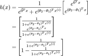
当类别数 $\textstyle k = 2$ 时，softmax 回归退化为 logistic 回归。这表明 softmax 回归是 logistic 回归的一般形式。具体地说，当 $\textstyle k = 2$ 时，softmax 回归的假设函数为：

$\begin{align}h_\theta(x) &=\frac{1}{ e^{\theta_1^Tx} + e^{ \theta_2^T x^{(i)} } }\begin{bmatrix}e^{ \theta_1^T x } \\e^{ \theta_2^T x }\end{bmatrix}\end{align}$

利用softmax回归参数冗余的特点，我们令 $\textstyle \psi = \theta_1$ ，并且从两个参数向量中都减去向量 $\textstyle \theta_1$ ，得到:

$\begin{align}h(x) &=\frac{1}{ e^{\vec{0}^Tx} + e^{ (\theta_2-\theta_1)^T x^{(i)} } }\begin{bmatrix}e^{ \vec{0}^T x } \\e^{ (\theta_2-\theta_1)^T x }\end{bmatrix} \\&=\begin{bmatrix}\frac{1}{ 1 + e^{ (\theta_2-\theta_1)^T x^{(i)} } } \\\frac{e^{ (\theta_2-\theta_1)^T x }}{ 1 + e^{ (\theta_2-\theta_1)^T x^{(i)} } }\end{bmatrix} \\&=\begin{bmatrix}\frac{1}{ 1 + e^{ (\theta_2-\theta_1)^T x^{(i)} } } \\1 - \frac{1}{ 1 + e^{ (\theta_2-\theta_1)^T x^{(i)} } } \\\end{bmatrix}\end{align}$

因此，用 $\textstyle \theta'$ 来表示 $\textstyle \theta_2-\theta_1$ ，我们就会发现 softmax 回归器预测其中一个类别的概率为 $\textstyle \frac{1}{ 1 + e^{ (\theta')^T x^{(i)} } }$ ，另一个类别概率的为 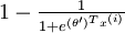$\textstyle 1 - \frac{1}{ 1 + e^{ (\theta')^T x^{(i)} } }$ ，这与 logistic回归是一致的。

Softmax 回归 vs. k 个二元分类器

如果你在开发一个音乐分类的应用，需要对k种类型的音乐进行识别，那么是选择使用 softmax 分类器呢，还是使用 logistic 回归算法建立 k 个独立的二元分类器呢？

这一选择取决于你的类别之间是否互斥，例如，如果你有四个类别的音乐，分别为：古典音乐、乡村音乐、摇滚乐和爵士乐，那么你可以假设每个训练样本只会被打上一个标签（即：一首歌只能属于这四种音乐类型的其中一种），此时你应该使用类别数 $k = 4$ 的softmax回归。（如果在你的数据集中，有的歌曲不属于以上四类的其中任何一类，那么你可以添加一个“其他类”，并将类别数 $k$ 设为5。）

如果你的四个类别如下：人声音乐、舞曲、影视原声、流行歌曲，那么这些类别之间并不是互斥的。例如：一首歌曲可以来源于影视原声，同时也包含人声。这种情况下，使用4个二分类的 logistic 回归分类器更为合适。这样，对于每个新的音乐作品，我们的算法可以分别判断它是否属于各个类别。

现在我们来看一个计算视觉领域的例子，你的任务是将图像分到三个不同类别中。(i) 假设这三个类别分别是：室内场景、户外城区场景、户外荒野场景。你会使用sofmax回归还是 3个logistic 回归分类器呢？ (ii) 现在假设这三个类别分别是室内场景、黑白图片、包含人物的图片，你又会选择 softmax 回归还是多个 logistic 回归分类器呢？

在第一个例子中，三个类别是互斥的，因此更适于选择softmax回归分类器。而在第二个例子中，建立三个独立的 logistic回归分类器更加合适。

中英文对照

Softmax回归 Softmax Regression

有监督学习 supervised learning

无监督学习 unsupervised learning

深度学习 deep learning

logistic回归 logistic regression

截距项 intercept term

二元分类 binary classification

类型标记 class labels

估值函数/估计值 hypothesis

代价函数 cost function

多元分类 multi-class classification

权重衰减 weight decay

中文译者

曾俊瑀（knighterzjy@gmail.com）, 王方（fangkey@gmail.com），王文中（wangwenzhong@ymail.com）

Softmax算法：逻辑回归的扩展

分类：统计机器学习算法理论 2013-08-09 23:35 375人阅读评论(0) 收藏举报

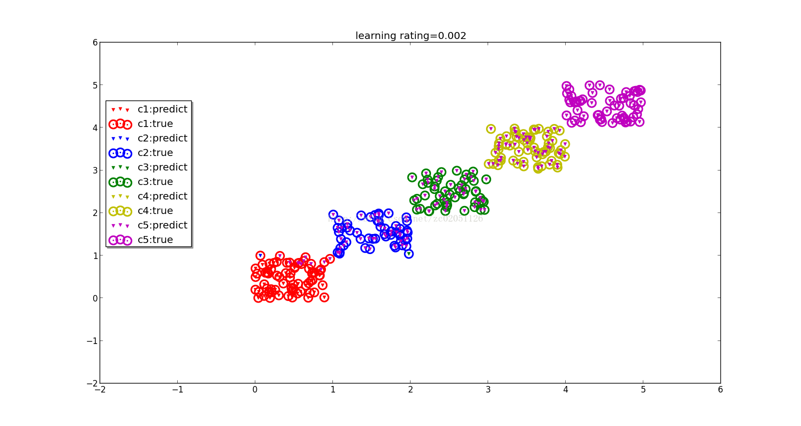
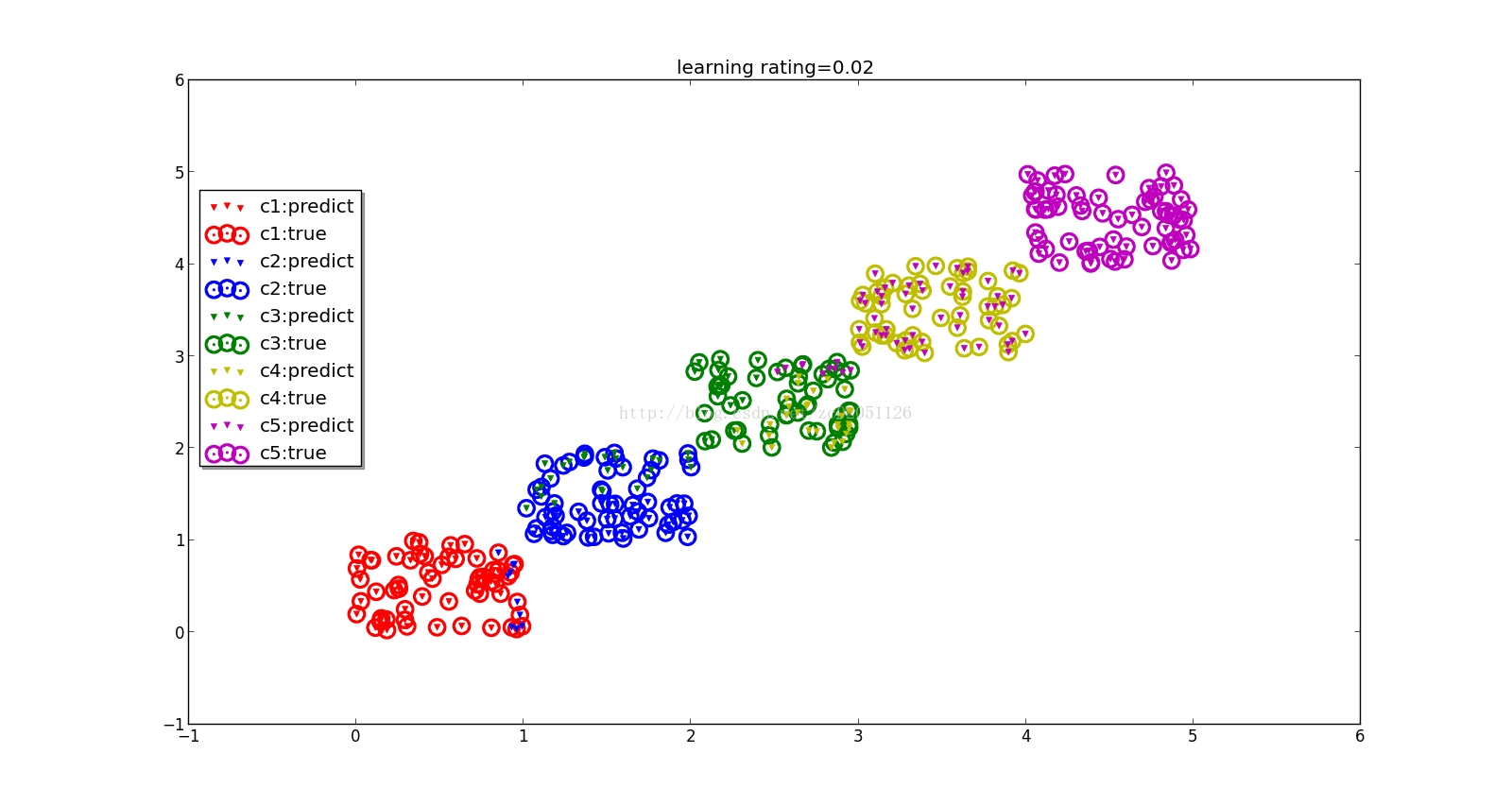
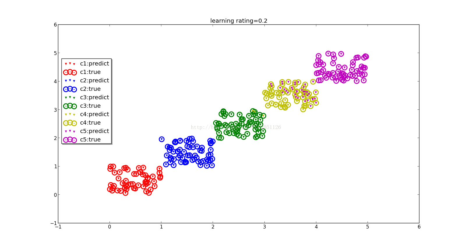
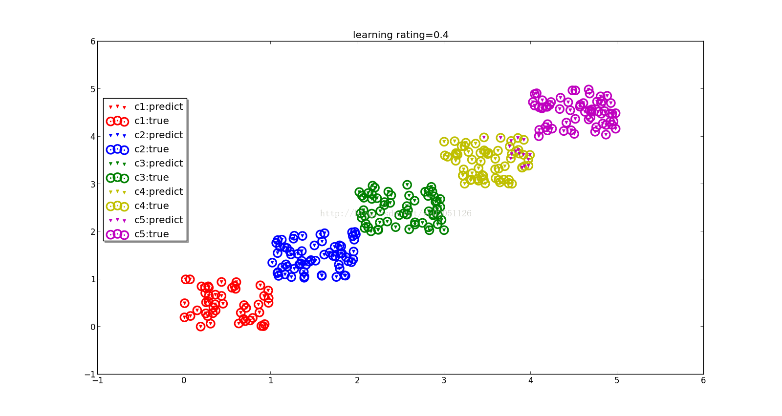
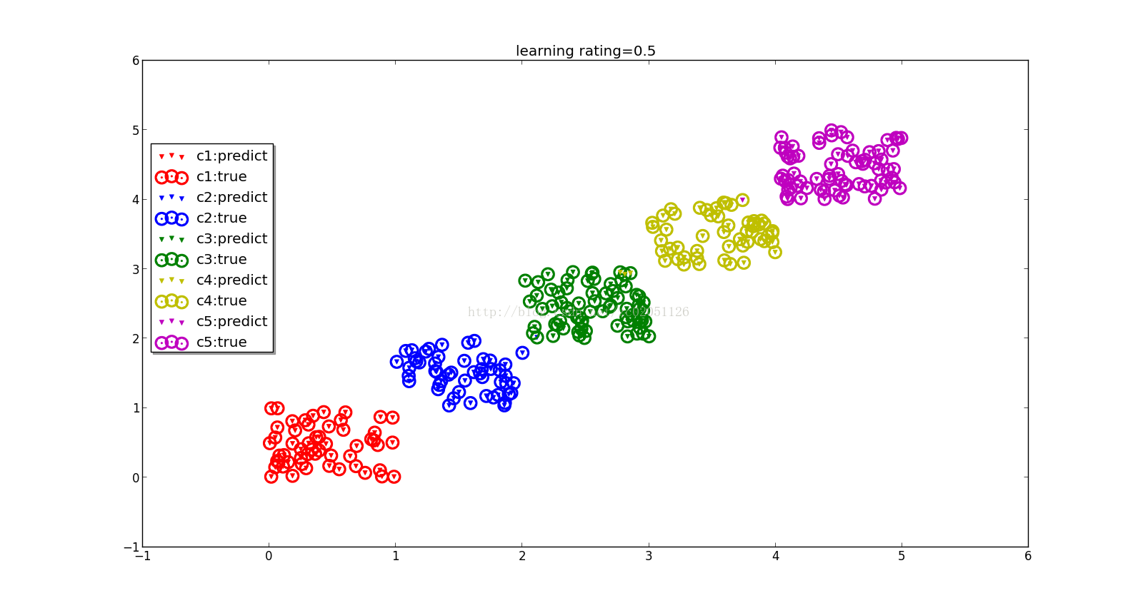
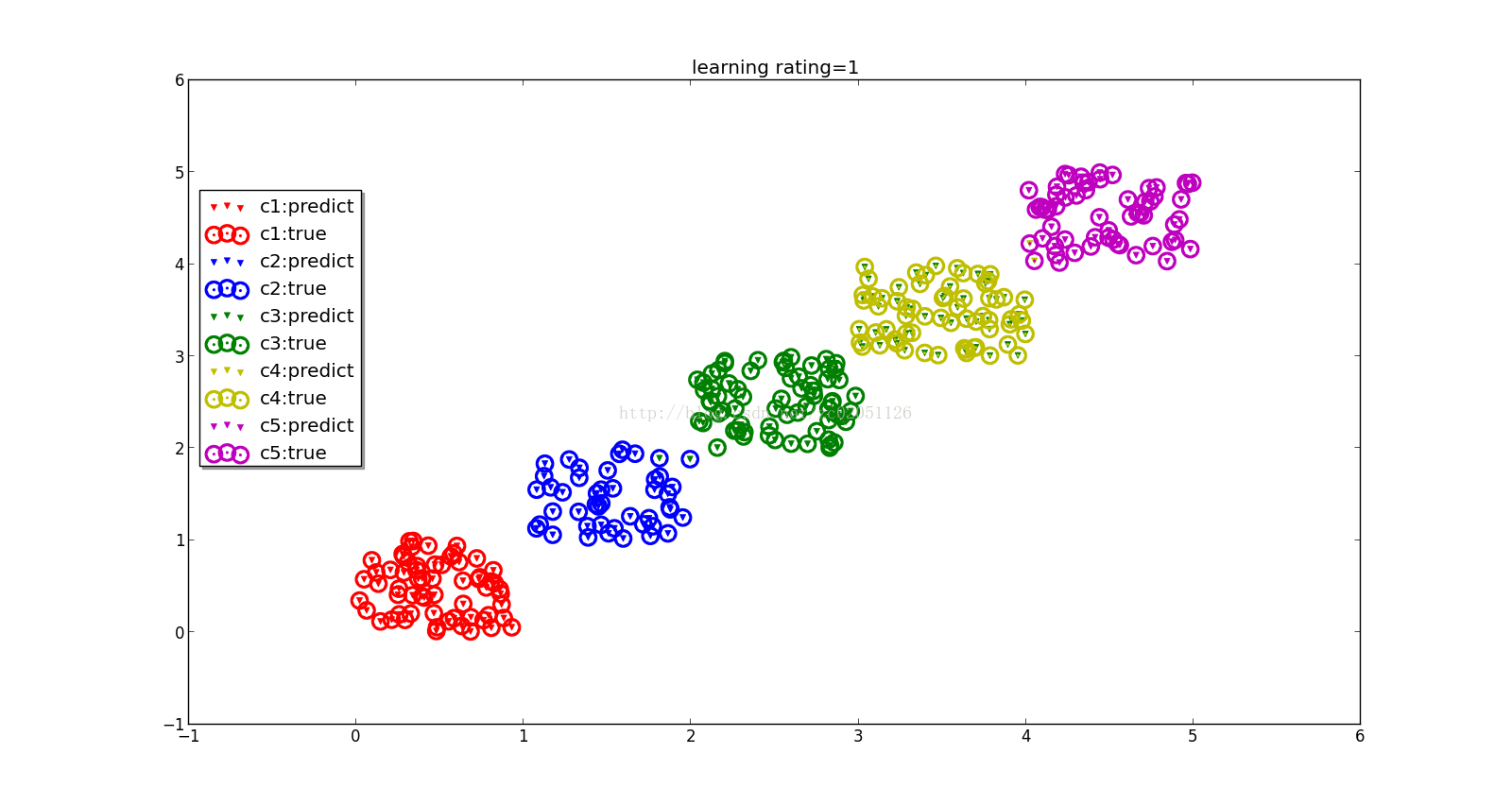
终于实现了逻辑回归的扩展版本，训练方法采用梯度下降法，这种方法对学习率的要求比较高，不同的学习率可能导致结果大相径庭。见相关图

参考资料：http://deeplearning.stanford.edu/wiki/index.php/Softmax%E5%9B%9E%E5%BD%92

Python代码如下：

[python]view plaincopy 
    
 
    
 import numpy as np  
 import matplotlib.pylab as plt  
 import copy  
 from scipy.linalg import norm  
 from math import pow  
 from scipy.optimize import fminbound,minimize  
 import random  
 def _dot(a, b):  
     mat_dot = np.dot(a, b)  
     return np.exp(mat_dot)  
 def condProb(theta, thetai, xi):  
     numerator = _dot(thetai, xi.transpose())  
           
     denominator = _dot(theta, xi.transpose())  
     denominator = np.sum(denominator, axis=0)  
     p = numerator / denominator  
     return p  
 def costFunc(alfa, *args):  
     i = args[2]  
     original_thetai = args[0]  
     delta_thetai = args[1]  
     x = args[3]  
     y = args[4]  
     lamta = args[5]  
       
     labels = set(y)  
     thetai = original_thetai  
     thetai[i, :] = thetai[i, :] - alfa * delta_thetai  
     k = 0  
     sum_log_p = 0.0  
     for label in labels:  
         index = y == label  
         xi = x[index]  
         p = condProb(original_thetai,thetai[k, :], xi)  
         log_p = np.log10(p)  
         sum_log_p = sum_log_p + log_p.sum()  
         k = k + 1  
     r = -sum_log_p / x.shape[0]+ (lamta / 2.0) * pow(norm(thetai),2)  
     #print r ,alfa  
   
     return r  
 class Softmax:  
     def __init__(self, alfa, lamda, feature_num, label_mum, run_times = 500, col = 1e-6):  
         self.alfa = alfa  
         self.lamda = lamda  
         self.feature_num = feature_num  
         self.label_num = label_mum  
         self.run_times = run_times  
         self.col = col  
         self.theta = np.random.random((label_mum, feature_num + 1))+1.0  
     def oneDimSearch(self, original_thetai,delta_thetai,i,x,y ,lamta):  
         res = minimize(costFunc, 0.0, method = 'Powell', args =(original_thetai,delta_thetai,i,x,y ,lamta))  
         return res.x  
     def train(self, x, y):  
         tmp = np.ones((x.shape[0], x.shape[1] + 1))  
         tmp[:,1:tmp.shape[1]] = x  
         x = tmp  
         del tmp  
         labels = set(y)  
         self.errors = []  
         old_alfa = self.alfa  
         for kk in range(0, self.run_times):  
             i = 0  
               
             for label in labels:  
                 tmp_theta = copy.deepcopy(self.theta)  
                 one = np.zeros(x.shape[0])  
                 index = y == label  
                 one[index] = 1.0  
                 thetai = np.array([self.theta[i, :]])  
                 prob = self.condProb(thetai, x)  
                 prob = np.array([one - prob])  
                 prob = prob.transpose()  
                 delta_thetai = - np.sum(x * prob, axis = 0)/ x.shape[0] + self.lamda * self.theta[i, :]  
                 #alfa = self.oneDimSearch(self.theta,delta_thetai,i,x,y ,self.lamda)#一维搜索法寻找最优的学习率，没有实现  
                 self.theta[i,:] = self.theta[i,:] - self.alfa * np.array([delta_thetai])  
                 i = i + 1  
             self.errors.append(self.performance(tmp_theta))  
           
     def performance(self, tmp_theta):  
         return norm(self.theta - tmp_theta)   
     def dot(self, a, b):  
         mat_dot = np.dot(a, b)  
         return np.exp(mat_dot)  
     def condProb(self, thetai, xi):  
         numerator = self.dot(thetai, xi.transpose())  
           
         denominator = self.dot(self.theta, xi.transpose())  
         denominator = np.sum(denominator, axis=0)  
         p = numerator[0] / denominator  
         return p  
     def predict(self, x):  
         tmp = np.ones((x.shape[0], x.shape[1] + 1))  
         tmp[:,1:tmp.shape[1]] = x  
         x = tmp  
         row = x.shape[0]  
         col = self.theta.shape[0]  
         pre_res = np.zeros((row, col))  
         for i in range(0, row):  
             xi = x[i, :]  
             for j in range(0, col):  
                 thetai = self.theta[j, :]  
                 p = self.condProb(np.array([thetai]), np.array([xi]))  
                 pre_res[i, j] = p  
         r = []  
         for i in range(0, row):  
             tmp = []  
             line = pre_res[i, :]  
             ind = line.argmax()  
             tmp.append(ind)  
             tmp.append(line[ind])  
             r.append(tmp)  
         return np.array(r)  
     def evaluate(self):  
         pass  
 def samples(sample_num, feature_num, label_num):  
     n = int(sample_num / label_num)  
     x = np.zeros((n*label_num, feature_num))  
     y = np.zeros(n*label_num, dtype=np.int)  
     for i in range(0, label_num):  
         x[i*n : i*n + n, :] = np.random.random((n, feature_num)) + i  
         y[i*n : i*n + n] = i  
     return [x, y]  
 def save(name, x, y):  
     writer = open(name, 'w')  
     for i in range(0, x.shape[0]):  
         for j in range(0, x.shape[1]):  
             writer.write(str(x[i,j]) + ' ')  
         writer.write(str(y[i])+ '\n')  
     writer.close()  
 def load(name):  
     x = []  
     y = []  
     for line in open(name, 'r'):  
         ele = line.split(' ')  
         tmp = []  
         for i in range(0, len(ele) - 1):  
             tmp.append(float(ele[i]))  
         x.append(tmp)  
         y.append(int(ele[len(ele) - 1]))  
     return [x, y]  
 def plotRes(pre, real, test_x,l):  
     s = set(pre)  
     col = ['r','b','g','y','m']  
     fig = plt.figure()  
       
     ax = fig.add_subplot(111)  
     for i in range(0, len(s)):  
         index1 = pre == i  
         index2 = real == i  
         x1 = test_x[index1, :]  
         x2 = test_x[index2, :]  
         ax.scatter(x1[:,0],x1[:,1],color=col[i],marker='v',linewidths=0.5)  
         ax.scatter(x2[:,0],x2[:,1],color=col[i],marker='.',linewidths=12)  
     plt.title('learning rating='+str(l))  
     plt.legend(('c1:predict','c1:true',\  
                 'c2:predict','c2:true',  
                 'c3:predict','c3:true',  
                 'c4:predict','c4:true',  
                 'c5:predict','c5:true'), shadow = True, loc = (0.01, 0.4))  
     plt.show()    
 if __name__ == '__main__':  
     #[x, y] = samples(1000, 2, 5)  
     #save('data.txt', x, y)  
     [x, y] = load('data.txt')  
     index= range(0, len(x))  
     random.shuffle(index)  
     x = np.array(x)  
     y = np.array(y)  
     x_train = x[index[0:700],:]  
     y_train = y[index[0:700]]  
     softmax = Softmax(0.4, 0.0, 2, 5)#这里讲第二个参数设置为0.0，即不用正则化，因为模型中没有高次项，用正则化反而使效果变差  
     softmax.train(x_train, y_train)  
     x_test = x[index[700:1000],:]  
     y_test = y[index[700:1000]]  
     r= softmax.predict(x_test)  
     plotRes(r[:,0],y_test,x_test,softmax.alfa)  
     t = r[:,0] != y_test  
     o = np.zeros(len(t))  
     o[t] = 1  
     err = sum(o)  
       
 
    
  

计算结果如下，如下面几幅图中看到，随着学习率的变大，分类效果越来越好，当大到一定程度，如为1时效果又变差，所以如何学则学习率是关键，该代码中用到的数据可以自动生成。

haoji007

关注

0
点赞
踩
0

收藏

觉得还不错? 一键收藏
0
评论
Softmax算法：逻辑回归的扩展

Softmax回归Contents [hide]1 简介2 代价函数3 Softmax回归模型参数化的特点4 权重衰减5 Softmax回归与Logistic 回归的关系6 Softmax 回归 vs. k 个二元分类器7 中英文对照8 中文译者简介在本节中，我们介绍Softmax回归模型，该模型是logis
复制链接

扫一扫