caffe 提取特征并可视化（已测试可执行）及在线可视化

最新推荐文章于 2023-03-05 20:38:45 发布

haoji007

最新推荐文章于 2023-03-05 20:38:45 发布

阅读量960

点赞数

分类专栏：【Caffe 及应用实例】【深度学习--应用实例】

【Caffe 及应用实例】同时被 2 个专栏收录

246 篇文章 7 订阅

订阅专栏

【深度学习--应用实例】

87 篇文章 11 订阅

订阅专栏

caffe 提取特征并可视化（已测试可执行）及在线可视化

转载 2015年12月26日 21:24:52

网络结构在线可视化工具

http://ethereon.github.io/netscope/#/editor

参考主页：

caffe 可视化的资料可在百度云盘下载
链接: http://pan.baidu.com/s/1jIRJ6mU
提取密码：xehi

http://cs.stanford.edu/people/karpathy/cnnembed/

http://lijiancheng0614.github.io/2015/08/21/2015_08_21_CAFFE_Features/
http://nbviewer.ipython.org/github/BVLC/caffe/blob/master/examples/00-classification.ipynb
http://www.cnblogs.com/platero/p/3967208.html
http://caffe.berkeleyvision.org/gathered/examples/feature_extraction.html
http://caffecn.cn/?/question/21

caffe程序是由c++语言写的，本身是不带数据可视化功能的。只能借助其它的库或接口，如opencv, python或matlab。使用python接口来进行可视化，因为python出了个比较强大的东西：ipython notebook, 最新版本改名叫jupyter notebook，它能将python代码搬到浏览器上去执行，以富文本方式显示，使得整个工作可以以笔记的形式展现、存储，对于交互编程、学习非常方便。

使用CAFFE（ http://caffe.berkeleyvision.org ）运行CNN网络，并提取出特征，将其存储成lmdb以供后续使用，亦可以对其可视化

使用已训练好的模型进行图像分类在 http://nbviewer.ipython.org/github/BVLC/caffe/blob/master/example/00-classification.ipynb 中已经很详细地介绍了怎么使用已训练好的模型对测试图像进行分类了。由于CAFFE不断更新，这个页面的内容和代码也会更新。以下只记录当前能运行的主要步骤。下载CAFFE，并安装相应的dependencies，说白了就是配置好caffe。

1. 下载CAFFE，并安装相应的dependencies，说白了就是配置好caffe运行环境。

2. 配置好 python ipython notebook,具体可参考网页: 

 
 1
2
3
4

http://blog.csdn.net/jiandanjinxin/article/details/50409448
3. 在caffe_root下运行./scripts/download_model_binary.py models/bvlc_reference_caffenet获得预训练的CaffeNet。获取CaffeNet网络并储存到models/bvlc_reference_caffenet目录下。

cd caffe-root
python ./scripts/download_model_binary.py models/bvlc_reference_caffenet
 
 1
2

  4. 在python文件夹下进入ipython模式（或python，但需要把部分代码注释掉）运行以下代码        

 
 1
2

cd ./python  #（×）  后面会提到
ipython notebook 
 
 1
2

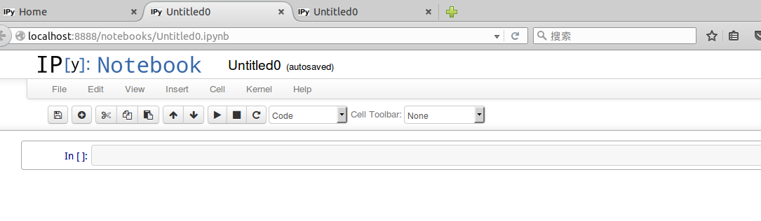
在命令行输入 ipython notebook,会出现一下画面
这里写图片描述

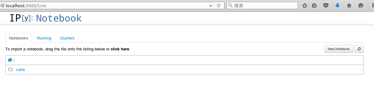
  接着 点击  New Notebook，就可以输入代码，按 shift+enter 执行

 
 1
2

这里写图片描述

python环境不能单独配置，必须要先编译好caffe，才能编译python环境。

安装jupyter

sudo pip install jupyter
 
 1

安装成功后，运行notebook

jupyter notebook
 
 1

  输入下面代码：

 
 1
2

import numpy as np
import matplotlib.pyplot as plt
%matplotlib inline

# Make sure that caffe is on the python path:
caffe_root = '../'  
# this file is expected to be in {caffe_root}/examples
#这里注意路径一定要设置正确,记得前后可能都有“/”,路径的使用是
#{caffe_root}/examples,记得 caffe-root 中的 python 文件夹需要包括 caffe 文件夹。

#caffe_root = '/home/bids/caffer-root/' #为何设置为具体路径反而不能运行呢

import sys
sys.path.insert(0, caffe_root + 'python')
import caffe #把 ipython 的路径改到指定的地方(这里是说刚开始在终端输入ipython notebook命令时，一定要确保是在包含caffe的python文件夹，这就是上面代码（×）),以便可以调入 caffe 模块,如果不改路径,import 这个指令只会在当前目录查找,是找不到 caffe 的。

plt.rcParams['figure.figsize'] = (10, 10)
plt.rcParams['image.interpolation'] = 'nearest'
plt.rcParams['image.cmap'] = 'gray'
#显示的图表大小为 10,图形的插值是以最近为原则,图像颜色是灰色

import os
if not os.path.isfile(caffe_root + 'models/bvlc_reference_caffenet/bvlc_reference_caffenet.caffemodel'):
    print("Downloading pre-trained CaffeNet model...")
    !../scripts/download_model_binary.py ../models/bvlc_reference_caffenet

#设置网络为测试阶段，并加载网络模型prototxt和数据平均值mean_npy

caffe.set_mode_cpu()# 采用CPU运算
net = caffe.Net(caffe_root + 'models/bvlc_reference_caffenet/deploy.prototxt',caffe_root + 'models/bvlc_reference_caffenet/bvlc_reference_caffenet.caffemodel',caffe.TEST)

# input preprocessing: 'data' is the name of the input blob == net.inputs[0]
transformer = caffe.io.Transformer({'data': net.blobs['data'].data.shape})
transformer.set_transpose('data', (2,0,1))
transformer.set_mean('data', np.load(caffe_root + 'python/caffe/imagenet/ilsvrc_2012_mean.npy').mean(1).mean(1)) 
# mean pixel，ImageNet的均值
transformer.set_raw_scale('data', 255) 
# the reference model operates on images in [0,255] range instead of [0,1]。参考模型运行在【0,255】的灰度,而不是【0,1】

transformer.set_channel_swap('data', (2,1,0))  

# the reference model has channels in BGR order instead of RGB，因为参考模型本来频道是 BGR,所以要将RGB转换

# set net to batch size of 50
net.blobs['data'].reshape(50,3,227,227)

#加载测试图片，并预测分类结果。

net.blobs['data'].data[...] = transformer.preprocess('data', caffe.io.load_image(caffe_root + 'examples/images/cat.jpg'))
out = net.forward()
print("Predicted class is #{}.".format(out['prob'][0].argmax()))

plt.imshow(transformer.deprocess('data', net.blobs['data'].data[0]))

# load labels,加载标签，并输出top_k
imagenet_labels_filename = caffe_root + 'data/ilsvrc12/synset_words.txt'
try:
    labels = np.loadtxt(imagenet_labels_filename, str, delimiter='\t')
except:
    !../data/ilsvrc12/get_ilsvrc_aux.sh
    labels = np.loadtxt(imagenet_labels_filename, str, delimiter='\t')
# sort top k predictions from softmax output

top_k = net.blobs['prob'].data[0].flatten().argsort()[-1:-6:-1]
print labels[top_k]


# CPU 与 GPU 比较运算时间
# CPU mode

net.forward()  # call once for allocation
%timeit net.forward()

# GPU mode
caffe.set_device(0)
caffe.set_mode_gpu()
net.forward()  # call once for allocation
%timeit net.forward()

#****提取特征并可视化****

#网络的特征存储在net.blobs，参数和bias存储在net.params，以下代码输出每一层的名称和大小。这里亦可手动把它们存储下来。

[(k, v.data.shape) for k, v in net.blobs.items()]

#显示出各层的参数和形状,第一个是批次,第二个 feature map 数目,第三和第四是每个神经元中图片的长和宽,可以看出,输入是 227*227 的图片,三个频道,卷积是 32 个卷积核卷三个频道,因此有 96 个 feature map

[(k, v[0].data.shape) for k, v in net.params.items()]
#输出:一些网络的参数

#**可视化的辅助函数**
# take an array of shape (n, height, width) or (n, height, width, channels)用一个格式是(数量,高,宽)或(数量,高,宽,频道)的阵列
# and visualize each (height, width) thing in a grid of size approx. sqrt(n) by sqrt(n)每个可视化的都是在一个由一个个网格组成

def vis_square(data, padsize=1, padval=0):
    data -= data.min()
    data /= data.max()

    # force the number of filters to be square
    n = int(np.ceil(np.sqrt(data.shape[0])))
    padding = ((0, n ** 2 - data.shape[0]), (0, padsize), (0, padsize)) + ((0, 0),) * (data.ndim - 3)
    data = np.pad(data, padding, mode='constant', constant_values=(padval, padval))

    # tile the filters into an image
    data = data.reshape((n, n) + data.shape[1:]).transpose((0, 2, 1, 3) + tuple(range(4, data.ndim + 1)))
    data = data.reshape((n * data.shape[1], n * data.shape[3]) + data.shape[4:])

    plt.imshow(data)


#根据每一层的名称，选择需要可视化的层，可以可视化filter（参数）和output（特征）
# the parameters are a list of [weights, biases],各层的特征，第一个卷积层，共96个过滤器
filters = net.params['conv1'][0].data
vis_square(filters.transpose(0, 2, 3, 1))
#使用 ipt.show()观看图像

#过滤后的输出,96 张 featuremap
feat = net.blobs['conv1'].data[4, :96]
vis_square(feat, padval=1)
#使用 ipt.show()观看图像:

feat = net.blobs['conv1'].data[0, :36]
vis_square(feat, padval=1)


#第二个卷积层:有 128 个滤波器,每个尺寸为 5X5X48。我们只显示前面 48 个滤波器,每一个滤波器为一行。输入:
filters = net.params['conv2'][0].data
vis_square(filters[:48].reshape(48**2, 5, 5))
#使用 ipt.show()观看图像:

#第二层输出 256 张 feature,这里显示 36 张。输入:
feat = net.blobs['conv2'].data[4, :36]
vis_square(feat, padval=1)
#使用 ipt.show()观看图像

feat = net.blobs['conv2'].data[0, :36]
vis_square(feat, padval=1)

#第三个卷积层:全部 384 个 feature map,输入:
feat = net.blobs['conv3'].data[4]
vis_square(feat, padval=0.5)
#使用 ipt.show()观看图像:

#第四个卷积层:全部 384 个 feature map,输入:
feat = net.blobs['conv4'].data[4]
vis_square(feat, padval=0.5)
#使用 ipt.show()观看图像:

#第五个卷积层:全部 256 个 feature map,输入:
feat = net.blobs['conv5'].data[4]
vis_square(feat, padval=0.5)
#使用 ipt.show()观看图像:

#第五个 pooling 层:我们也可以观察 pooling 层,输入:
feat = net.blobs['pool5'].data[4]
vis_square(feat, padval=1)
#使用 ipt.show()观看图像:

#用caffe 的python接口提取和保存特征比较方便。
features = net.blobs['conv5'].data  # 提取卷积层 5 的特征
np.savetxt('conv5_feature.txt', features) # 将特征存储到本文文件中


#然后我们看看第六层(第一个全连接层)输出后的直方分布:
feat = net.blobs['fc6'].data[4]
plt.subplot(2, 1, 1)
plt.plot(feat.flat)
plt.subplot(2, 1, 2)
_ = plt.hist(feat.flat[feat.flat > 0], bins=100)
#使用 ipt.show()观看图像:

#第七层（第二个全连接层）输出后的直方分布:可以看出值的分布没有这么平均了。
feat = net.blobs['fc7'].data[4]
plt.subplot(2, 1, 1)
plt.plot(feat.flat)
plt.subplot(2, 1, 2)
_ = plt.hist(feat.flat[feat.flat > 0], bins=100)
#使用 ipt.show()观看图像:

#The final probability output, prob
feat = net.blobs['prob'].data[0]
plt.plot(feat.flat)


#最后看看标签:Let's see the top 5 predicted labels.
# load labels
imagenet_labels_filename = caffe_root + 'data/ilsvrc12/synset_words.txt'
try:
    labels = np.loadtxt(imagenet_labels_filename, str, delimiter='\t')
except:
    !../data/ilsvrc12/get_ilsvrc_aux.sh
    labels = np.loadtxt(imagenet_labels_filename, str, delimiter='\t')

# sort top k predictions from softmax output
top_k = net.blobs['prob'].data[0].flatten().argsort()[-1:-6:-1]
print labels[top_k]

 
 1
2
3
4
5
6
7
8
9
10
11
12
13
14
15
16
17
18
19
20
21
22
23
24
25
26
27
28
29
30
31
32
33
34
35
36
37
38
39
40
41
42
43
44
45
46
47
48
49
50
51
52
53
54
55
56
57
58
59
60
61
62
63
64
65
66
67
68
69
70
71
72
73
74
75
76
77
78
79
80
81
82
83
84
85
86
87
88
89
90
91
92
93
94
95
96
97
98
99
100
101
102
103
104
105
106
107
108
109
110
111
112
113
114
115
116
117
118
119
120
121
122
123
124
125
126
127
128
129
130
131
132
133
134
135
136
137
138
139
140
141
142
143
144
145
146
147
148
149
150
151
152
153
154
155
156
157
158
159
160
161
162
163
164
165
166
167
168
169
170
171
172
173
174
175
176
177
178
179
180
181
182
183
184
185
186
187
188
189
190
191
192
193
194
195
196
197

备注：用 caffe 的 python 接口提取和保存特征到text文本下

features = net.blobs['conv5'].data  # 提取卷积层 5 的特征
np.savetxt('conv5_feature.txt', features) # 将特征存储到本文文件中
 
 1
2

现在Caffe的Matlab接口 (matcaffe3) 和python接口都非常强大, 可以直接提取任意层的feature map以及parameters, 所以本文仅仅作为参考, 更多最新的信息请参考:
http://caffe.berkeleyvision.org/tutorial/interfaces.html

提取特征并储存
CAFFE提供了一个提取特征的tool，见 http://caffe.berkeleyvision.org/gathered/examples/feature_extraction.html 。

数据模型与准备
安装好Caffe后，在examples/images文件夹下有两张示例图像，本文即在这两张图像上，用Caffe提供的预训练模型，进行特征提取，并进行可视化。

1. 选择需要特征提取的图像
./examples/_temp

(1) 进入caffe根目录(本文中caffe的根目录都为caffe-root)，创建临时文件夹，用于存放所需要的临时文件

mkdir examples/_temp
 
 1

(2) 根据examples/images文件夹中的图片，创建包含图像列表的txt文件，并添加标签（0）

find `pwd`/examples/images -type f -exec echo {} \; > examples/_temp/temp.txt
sed "s/$/ 0/" examples/_temp/temp.txt > examples/_temp/file_list.txt
 
 1
2

(3) 执行下列脚本，下载imagenet12图像均值文件，在后面的网络结构定义prototxt文件中，需要用到该文件（data/ilsvrc212/imagenet_mean.binaryproto）.下载模型以及定义prototxt。

sh ./data/ilsvrc12/get_ilsvrc_aux.sh
 
 1

(4) 将网络定义prototxt文件复制到_temp文件夹下

cp examples/feature_extraction/imagenet_val.prototxt examples/_temp
 
 1

使用特征文件进行可视化
参考 http://www.cnblogs.com/platero/p/3967208.html 和 lmdb的文档 https://lmdb.readthedocs.org/en/release ，读取lmdb文件，然后转换成mat文件，再用matlab调用mat进行可视化。

使用caffe的 extract_features.bin 工具提取出的图像特征存为lmdb格式，为了方便观察特征，我们将利用下列两个python脚本将图像转化为matlab的.mat格式（请先安装caffe的python依赖库）。extract_features.bin的运行参数为

extract_features.bin $MODEL $PROTOTXT $LAYER $LMDB_OUTPUT_PATH $BATCHSIZE
 
 1

上面不是执行代码，只是运行参数，不需要执行上式。

下面给出第一个例子是提取特征并储存。

（1）安装CAFFE的python依赖库，并使用以下两个辅助文件把lmdb转换为mat。在caffe 根目录下创建feat_helper_pb2.py 和lmdb2mat.py，直接copy 下面的python程序即可。

cd caffe-root
sudo gedit  feat_helper_pb2.py
sudo gedit lmdb2mat.py
 
 1
2
3

需要添加的内容如下
feat_helper_pb2.py：

# Generated by the protocol buffer compiler.  DO NOT EDIT!

from google.protobuf import descriptor
from google.protobuf import message
from google.protobuf import reflection
from google.protobuf import descriptor_pb2
# @@protoc_insertion_point(imports)


DESCRIPTOR = descriptor.FileDescriptor(
  name='datum.proto',
  package='feat_extract',
  serialized_pb='\n\x0b\x64\x61tum.proto\x12\x0c\x66\x65\x61t_extract\"i\n\x05\x44\x61tum\x12\x10\n\x08\x63hannels\x18\x01 \x01(\x05\x12\x0e\n\x06height\x18\x02 \x01(\x05\x12\r\n\x05width\x18\x03 \x01(\x05\x12\x0c\n\x04\x64\x61ta\x18\x04 \x01(\x0c\x12\r\n\x05label\x18\x05 \x01(\x05\x12\x12\n\nfloat_data\x18\x06 \x03(\x02')


_DATUM = descriptor.Descriptor(
  name='Datum',
  full_name='feat_extract.Datum',
  filename=None,
  file=DESCRIPTOR,
  containing_type=None,
  fields=[
    descriptor.FieldDescriptor(
      name='channels', full_name='feat_extract.Datum.channels', index=0,
      number=1, type=5, cpp_type=1, label=1,
      has_default_value=False, default_value=0,
      message_type=None, enum_type=None, containing_type=None,
      is_extension=False, extension_scope=None,
      options=None),
    descriptor.FieldDescriptor(
      name='height', full_name='feat_extract.Datum.height', index=1,
      number=2, type=5, cpp_type=1, label=1,
      has_default_value=False, default_value=0,
      message_type=None, enum_type=None, containing_type=None,
      is_extension=False, extension_scope=None,
      options=None),
    descriptor.FieldDescriptor(
      name='width', full_name='feat_extract.Datum.width', index=2,
      number=3, type=5, cpp_type=1, label=1,
      has_default_value=False, default_value=0,
      message_type=None, enum_type=None, containing_type=None,
      is_extension=False, extension_scope=None,
      options=None),
    descriptor.FieldDescriptor(
      name='data', full_name='feat_extract.Datum.data', index=3,
      number=4, type=12, cpp_type=9, label=1,
      has_default_value=False, default_value="",
      message_type=None, enum_type=None, containing_type=None,
      is_extension=False, extension_scope=None,
      options=None),
    descriptor.FieldDescriptor(
      name='label', full_name='feat_extract.Datum.label', index=4,
      number=5, type=5, cpp_type=1, label=1,
      has_default_value=False, default_value=0,
      message_type=None, enum_type=None, containing_type=None,
      is_extension=False, extension_scope=None,
      options=None),
    descriptor.FieldDescriptor(
      name='float_data', full_name='feat_extract.Datum.float_data', index=5,
      number=6, type=2, cpp_type=6, label=3,
      has_default_value=False, default_value=[],
      message_type=None, enum_type=None, containing_type=None,
      is_extension=False, extension_scope=None,
      options=None),
  ],
  extensions=[
  ],
  nested_types=[],
  enum_types=[
  ],
  options=None,
  is_extendable=False,
  extension_ranges=[],
  serialized_start=29,
  serialized_end=134,
)

DESCRIPTOR.message_types_by_name['Datum'] = _DATUM

class Datum(message.Message):
  __metaclass__ = reflection.GeneratedProtocolMessageType
  DESCRIPTOR = _DATUM

  # @@protoc_insertion_point(class_scope:feat_extract.Datum)

# @@protoc_insertion_point(module_scope)
 
 1
2
3
4
5
6
7
8
9
10
11
12
13
14
15
16
17
18
19
20
21
22
23
24
25
26
27
28
29
30
31
32
33
34
35
36
37
38
39
40
41
42
43
44
45
46
47
48
49
50
51
52
53
54
55
56
57
58
59
60
61
62
63
64
65
66
67
68
69
70
71
72
73
74
75
76
77
78
79
80
81
82
83
84
85
86

./lmdb2mat.py

import lmdb
import feat_helper_pb2
import numpy as np
import scipy.io as sio
import time

def main(argv):
    lmdb_name = sys.argv[1]
    print "%s" % sys.argv[1]
    batch_num = int(sys.argv[2]);
    batch_size = int(sys.argv[3]);
    window_num = batch_num*batch_size;

    start = time.time()
    if 'db' not in locals().keys():
        db = lmdb.open(lmdb_name)
        txn= db.begin()
        cursor = txn.cursor()
        cursor.iternext()
        datum = feat_helper_pb2.Datum()

        keys = []
        values = []
        for key, value in enumerate( cursor.iternext_nodup()):
            keys.append(key)
            values.append(cursor.value())

    ft = np.zeros((window_num, int(sys.argv[4])))
    for im_idx in range(window_num):
        datum.ParseFromString(values[im_idx])
        ft[im_idx, :] = datum.float_data

    print 'time 1: %f' %(time.time() - start)
    sio.savemat(sys.argv[5], {'feats':ft})
    print 'time 2: %f' %(time.time() - start)
    print 'done!'

if __name__ == '__main__':
    import sys
    main(sys.argv)
 
 1
2
3
4
5
6
7
8
9
10
11
12
13
14
15
16
17
18
19
20
21
22
23
24
25
26
27
28
29
30
31
32
33
34
35
36
37
38
39
40

备注：用 caffe 的 python 接口提取和保存特征到text文本下

features = net.blobs['conv5'].data  # 提取卷积层 5 的特征
np.savetxt('conv5_feature.txt', features) # 将特征存储到本文文件中
 
 1
2

（2）在caffe 根目录下创建脚本文件extract_feature_example1.sh，并执行，将在examples/_temp文件夹下得到lmdb文件（features_conv1）和.mat文件（features_conv1.mat）

下载已经生成的模型

sudo gedit ./examples/imagenet/get_caffe_reference_imagenet_model.sh

 
 1
2

添加编辑内容如下：

#!/usr/bin/env sh
# This scripts downloads the caffe reference imagenet model
# for ilsvrc image classification and deep feature extraction

MODEL=caffe_reference_imagenet_model
CHECKSUM=bf44bac4a59aa7792b296962fe483f2b

if [ -f $MODEL ]; then
  echo "Model already exists. Checking md5..."
  os=`uname -s`
  if [ "$os" = "Linux" ]; then
    checksum=`md5sum $MODEL | awk '{ print $1 }'`
  elif [ "$os" = "Darwin" ]; then
    checksum=`cat $MODEL | md5`
  fi
  if [ "$checksum" = "$CHECKSUM" ]; then
    echo "Model checksum is correct. No need to download."
    exit 0
  else
    echo "Model checksum is incorrect. Need to download again."
  fi
fi

echo "Downloading..."

wget --no-check-certificate https://www.dropbox.com/s/n3jups0gr7uj0dv/$MODEL

echo "Done. Please run this command again to verify that checksum = $CHECKSUM."
 
 1
2
3
4
5
6
7
8
9
10
11
12
13
14
15
16
17
18
19
20
21
22
23
24
25
26
27
28

cd caffe-root
sudo gedit extract_feature_example1.sh
 
 1
2

需要添加的内容如下：

#!/usr/bin/env sh
# args for EXTRACT_FEATURE
TOOL=./build/tools
MODEL=./examples/imagenet/caffe_reference_imagenet_model #下载得到的caffe model
PROTOTXT=./examples/_temp/imagenet_val.prototxt # 网络定义
LAYER=conv1 # 提取层的名字，如提取fc7等
LEVELDB=./examples/_temp/features_conv1 # 保存的leveldb路径
BATCHSIZE=10

# args for LEVELDB to MAT
DIM=290400 # 需要手工计算feature长度
OUT=./examples/_temp/features_conv1.mat #.mat文件保存路径
BATCHNUM=1 # 有多少个batch， 本例只有两张图， 所以只有一个batch

$TOOL/extract_features.bin  $MODEL $PROTOTXT $LAYER $LEVELDB $BATCHSIZE lmdb
python lmdb2mat.py $LEVELDB $BATCHNUM  $BATCHSIZE $DIM $OUT
 
 1
2
3
4
5
6
7
8
9
10
11
12
13
14
15
16

执行之后，

cd caffe-root
sh extract_feature_example1.sh
 
 1
2

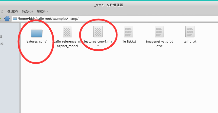
你会在/examples/_temp/ 下发现多了两个文件：文件夹 features_conv1，文件features_conv1.mat

这里写图片描述

如果执行出现lmdb2mat.py的相关问题，有可能是没有安装lmdb，可在caffe 根目录下执行下面的程式安装。具体问题具体分析。
Lmdb的安装

pip install lmdb
 
 1

特别备注：在执行一次 sh extract_feature_example1.sh 之后，在文件夹 _temp里面就会出现文件夹features_conv1和文件features_conv1.mat。若再次执行一次，会出现报错，可将文件夹 _temp中的文件夹features_conv1和文件features_conv1.mat 都删除，即可通过编译。

（3）. 参考UFLDL里的display_network函数，对mat文件里的特征进行可视化。
在/examples/_temp/ 中创建 display_network.m

cd ./examples/_temp/ 
sudo gedit display_network.m
 
 1
2

需要添加的内容如下：
display_network.m

function [h, array] = display_network(A, opt_normalize, opt_graycolor, cols, opt_colmajor)
% This function visualizes filters in matrix A. Each column of A is a
% filter. We will reshape each column into a square image and visualizes
% on each cell of the visualization panel. 
% All other parameters are optional, usually you do not need to worry
% about it.
% opt_normalize: whether we need to normalize the filter so that all of
% them can have similar contrast. Default value is true.
% opt_graycolor: whether we use gray as the heat map. Default is true.
% cols: how many columns are there in the display. Default value is the
% squareroot of the number of columns in A.
% opt_colmajor: you can switch convention to row major for A. In that
% case, each row of A is a filter. Default value is false.
warning off all

if ~exist('opt_normalize', 'var') || isempty(opt_normalize)
    opt_normalize= true;
end

if ~exist('opt_graycolor', 'var') || isempty(opt_graycolor)
    opt_graycolor= true;
end

if ~exist('opt_colmajor', 'var') || isempty(opt_colmajor)
    opt_colmajor = false;
end

% rescale
A = A - mean(A(:));

if opt_graycolor, colormap(gray); end

% compute rows, cols
[L M]=size(A);
sz=sqrt(L);
buf=1;
if ~exist('cols', 'var')
    if floor(sqrt(M))^2 ~= M
        n=ceil(sqrt(M));
        while mod(M, n)~=0 && n<1.2*sqrt(M), n=n+1; end
        m=ceil(M/n);
    else
        n=sqrt(M);
        m=n;
    end
else
    n = cols;
    m = ceil(M/n);
end

array=-ones(buf+m*(sz+buf),buf+n*(sz+buf));

if ~opt_graycolor
    array = 0.1.* array;
end


if ~opt_colmajor
    k=1;
    for i=1:m
        for j=1:n
            if k>M, 
                continue; 
            end
            clim=max(abs(A(:,k)));
            if opt_normalize
                array(buf+(i-1)*(sz+buf)+(1:sz),buf+(j-1)*(sz+buf)+(1:sz))=reshape(A(:,k),sz,sz)'/clim;
            else
                array(buf+(i-1)*(sz+buf)+(1:sz),buf+(j-1)*(sz+buf)+(1:sz))=reshape(A(:,k),sz,sz)'/max(abs(A(:)));
            end
            k=k+1;
        end
    end
else
    k=1;
    for j=1:n
        for i=1:m
            if k>M, 
                continue; 
            end
            clim=max(abs(A(:,k)));
            if opt_normalize
                array(buf+(i-1)*(sz+buf)+(1:sz),buf+(j-1)*(sz+buf)+(1:sz))=reshape(A(:,k),sz,sz)'/clim;
            else
                array(buf+(i-1)*(sz+buf)+(1:sz),buf+(j-1)*(sz+buf)+(1:sz))=reshape(A(:,k),sz,sz)';
            end
            k=k+1;
        end
    end
end

if opt_graycolor
    h=imagesc(array);
else
    h=imagesc(array,'EraseMode','none',[-1 1]);
end
axis image off

drawnow;

warning on all
 
 1
2
3
4
5
6
7
8
9
10
11
12
13
14
15
16
17
18
19
20
21
22
23
24
25
26
27
28
29
30
31
32
33
34
35
36
37
38
39
40
41
42
43
44
45
46
47
48
49
50
51
52
53
54
55
56
57
58
59
60
61
62
63
64
65
66
67
68
69
70
71
72
73
74
75
76
77
78
79
80
81
82
83
84
85
86
87
88
89
90
91
92
93
94
95
96
97
98
99
100
101

（4）在matlab里运行以下代码：
首先要进入 /examples/_temp/ 在执行下面的matlab程序。
在caffe 根目录下输入

cd ./examples/_temp/
matlab
 
 1
2

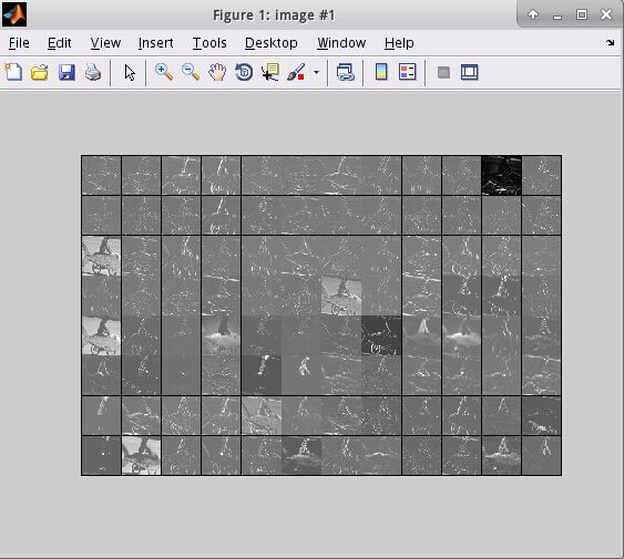
在matlab 中输入下面的命令

nsample = 3;
 num_output = 96; % conv1
% num_output = 256; % conv5
%num_output = 4096; % fc7

load features_conv1.mat
width = size(feats, 2);
nmap = width / num_output;

for i = 1 : nsample
    feat = feats(i, :);
    feat = reshape(feat, [nmap num_output]);
    figure('name', sprintf('image #%d', i));
    display_network(feat);
end
 
 1
2
3
4
5
6
7
8
9
10
11
12
13
14
15

执行之后将会出现一下结果：

这里写图片描述

在python中读取mat文件

在python中，使用scipy.io.loadmat()即可读取mat文件，返回一个dict()。

import scipy.io
matfile = 'features_conv1.mat'
data = scipy.io.loadmat(matfile)
 
 1
2
3

下面给出第二个例子：

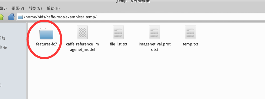
(1) 在caffe 根目录下创建脚本文件extract_feature_example2.sh，并执行，将在examples/_temp文件夹下得到lmdb文件（features_fc7）和.mat文件（features_fc7.mat）

cd caffe-root
sudo gedit extract_feature_example2.sh
 
 1
2

需要添加的内容如下：

#!/usr/bin/env sh
# args for EXTRACT_FEATURE
TOOL=./build/tools
MODEL=./models/bvlc_reference_caffenet/bvlc_reference_caffenet.caffemodel #下载得到的caffe model
PROTOTXT=./examples/_temp/imagenet_val.prototxt # 网络定义
LAYER=fc7 # 提取层的名字，如提取fc7等
LEVELDB=./examples/_temp/features_fc7 # 保存的leveldb路径
BATCHSIZE=10

# DIM=290400 # feature长度，conv1
# DIM=43264 # conv5
# args for LEVELDB to MAT
DIM=4096 # 需要手工计算feature长度
OUT=./examples/_temp/features_fc7.mat #.mat文件保存路径
BATCHNUM=1 # 有多少个batch， 本例只有两张图， 所以只有一个batch

$TOOL/extract_features.bin  $MODEL $PROTOTXT $LAYER $LEVELDB $BATCHSIZE lmdb
python lmdb2mat.py $LEVELDB $BATCHNUM  $BATCHSIZE $DIM $OUT
 
 1
2
3
4
5
6
7
8
9
10
11
12
13
14
15
16
17
18

执行之后，

cd caffe-root
sh extract_feature_example2.sh
 
 1
2

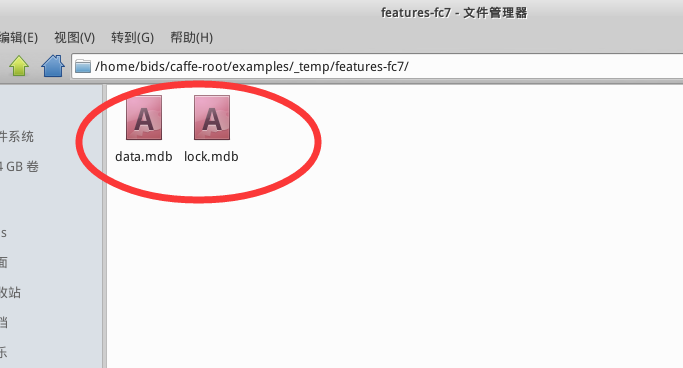
执行之后，你会在 examples/_temp/ 下多出一个文件夹 features-fc7，里面含有data.mdb, lock.mdb 两个文件,还会得到features-fc7.mat，如下图所示

这里写图片描述

（2）. 参考UFLDL里的display_network函数，对mat文件里的特征进行可视化。
在/examples/_temp/ 中创建 display_network.m

cd ./examples/_temp/ 
sudo gedit display_network.m
 
 1
2

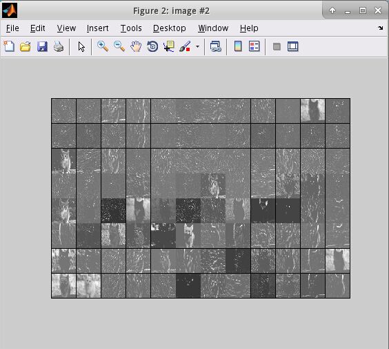
（3）在matlab里运行以下代码：
首先要进入 /examples/_temp/ 在执行下面的matlab程序。
在caffe 根目录下输入

cd ./examples/_temp/
matlab
 
 1
2

在matlab 中输入下面的命令

nsample = 2;
% num_output = 96; % conv1
% num_output = 256; % conv5
num_output = 4096; % fc7

load features_fc7.mat
width = size(feats, 2);
nmap = width / num_output;

for i = 1 : nsample
    feat = feats(i, :);
    feat = reshape(feat, [nmap num_output]);
    figure('name', sprintf('image #%d', i));
    display_network(feat);
end
 
 1
2
3
4
5
6
7
8
9
10
11
12
13
14
15

执行之后将会出现一下结果：

在python中读取mat文件

在python中，使用scipy.io.loadmat()即可读取mat文件，返回一个dict()。

import scipy.io
matfile = ‘features_fc7.mat’
data = scipy.io.loadmat(matfile)

使用自己的网络

只需把前面列出来的文件与参数修改成自定义的即可。

使用Model Zoo里的网络

根据 https://github.com/BVLC/caffe/wiki/Model-Zoo 的介绍，选择自己所需的网络，并下载到相应位置即可。

如VGG-16：

./scripts/download_model_from_gist.sh 211839e770f7b538e2d8
mv ./models/211839e770f7b538e2d8 ./models/VGG_ILSVRC_16_layers
./scripts/download_model_binary.py ./models/VGG_ILSVRC_16_layers

haoji007

关注

0
点赞
踩
0

收藏

觉得还不错? 一键收藏
0
评论
caffe 提取特征并可视化（已测试可执行）及在线可视化

caffe 提取特征并可视化（已测试可执行）及在线可视化转载 2015年12月26日 21:24:52标签：caffe/特征可视化/python网络结构在线可视化工具http://ethereon.github.io/netscope/#/editor参考主页：caffe 可视化的资料可在百度云盘下载链接: http:/
复制链接

扫一扫