


ImageNet Classification with Deep Convolutional NeuralNetwork
利用深度卷积神经网络进行ImageNet分类
Abstract
We trained a large, deep convolutionalneural network to classify the 1.2 million high-resolution images in theImageNet LSVRC-2010 contest into the 1000 different classes. On the test data,we achieved top-1 and top-5 error rates of 37.5% and 17.0% which isconsiderably better than the previous state-of-the-art. The neural network,which has 60 million parameters and 650,000 neurons, consists of fiveconvolutional layers, some of which are followed by max-pooling layers,
and three fully-connected layers with afinal 1000-way softmax. To make training faster, we used non-saturating neuronsand a very efficient GPU implementation of the convolution operation. To reduceoverfitting in the fully-connected layers we employed a recently-developedregularization method called “dropout” that proved to be very effective. Wealso entered a variant of this model in the ILSVRC-2012 competition andachieved a winning top-5 test error rate of 15.3%, compared to 26.2% achievedby the second-best entry.
摘要
我们训练了一个又大又深的卷积神经网络,来分类120万张图片,这些图都是从Imagenet 2010 竞赛库中的,1000个类别。在测试数据集上我们的第一判别错误率为37.5%,前五准确率17%,,比第二名要好很多。神经网络有着6000万的参数,和650000个神经元,由5个卷基层,其中一些附加上max-pooling层,3个全连阶层,和1000维的softmax层。为了使得训练更加快速我们使用不会饱和的神经元,以及高效的GPU来实现卷积,为了减少全连接层的过拟合,我们使用了一个最近较多使用的策略“dropout”,这种方法可以很高效。我们还参与了好多的ILSVRC 2012 的比赛并取得了前五错误5.3%,与第二名26.2%相比。
1 Introduction
Current approaches to object recognitionmake essential use of machine learning methods. To improve their performance,we can collect larger datasets, learn more powerful models, and use bettertechniques for preventing overfitting. Until recently, datasets of labeled imageswere relatively small — on the order of tens of thousands of images (e.g., NORB[16], Caltech-101/256 [8, 9], and CIFAR-10/100 [12]). imple recognition taskscan be solved quite well with datasets of this size, especially if they areaugmented with label-preserving transformations. For example, the currentbesterror rate on the MNIST digit-recognition task (<0.3%) approaches humanperformance [4]. But objects in realistic settings exhibit considerablevariability, so to learn to recognize them it is necessary to use much largertraining sets. And indeed, the shortcomings of small image datasets have beenwidely recognized (e.g., Pinto et al. [21]), but it has only recently becomepossible to collect labeled datasets with millions of images. The new largerdatasets include LabelMe [23], which consists of hundreds of thousands offully-segmented images, and ImageNet [6], which consists of over 15 millionlabeled high-resolution images in over 22,000 categories.
1介绍
现如今的对象识别方法都必不可少使用了机器学习方法。为了改善效果,我们收集了大量数据,学习了更加强大的模型,并使用了更好的技术来保证不会过拟合。直到最近,标注的数据集还是很小,大概是上万张左右(NORB,Caltech-101/256,Cifar-10/100),简单的识别可以用这种量级的数据集,特别是当他们在固定的标签条件下进行一定的图像转换,例如最近的最好的错误率达到(0.3%),接近人类水平。但是物体在现实世界出现时,会发生各种变化,所以学习如何识别他们时必须使用更大的训练集的,并且,的确大家已经很广泛地认识到小数据集的缺点,(pinto等人)但是直到最近,大型百万量级带标注数据集才成为可能,这些新数据集包括Labelme(包含十万张左右全分割的图像),还有Imagenet,包括了150万高分辨率标注图像,总共22000个类别
To learn about thousands of objects frommillions of images, we need a model with a large learning
capacity. However, the immense complexityof the object recognition task means that this problem cannot be specified evenby a dataset as large as ImageNet, so our model should also have lots
of prior knowledge to compensate for allthe data we don’t have. Convolutional neural networks
(CNNs) constitute one such class of models[16, 11, 13, 18, 15, 22, 26]. Their capacity can be controlled by varying theirdepth and breadth, and they also make strong and mostly correct assumptions aboutthe nature of images (namely, stationarity of statistics and locality of pixeldependencies).Thus, compared to standard feedforward neural networks withsimilarly-sized layers, CNNs havemuch fewer connections and parameters and sothey are easier to train, while their theoretically-best performance is likelyto be only slightly worse.
为了从百万级别的数据集学习上千个对象,我们需要一个大体量的模型。然而大规模的识别任务意味着,这个问题不能单独对待,即使在IMagenet这种大数据集合上,所以我们的模型需要先验知识来补偿我们所无法获取的数据。卷积神经网络就是我们需要的模型,它的体量可以通过调节深度和广度来控制,并且它还能对自然的图像进行很好的建模(很可能是正确的),例如稳定的统计学原理,还有局部像素之间的关联,因此,与标准的层节点数量相似反馈神经网络相比,CNN有更少的连接和参数,所以更容易训练,当然,我们仍不知道它理论上的最好的表现,可能是个微小的缺陷
Despite the attractive qualities of CNNs,and despite the relative efficiency of their local architecture,they have stillbeen prohibitively expensive to apply in large scale to high-resolution images.Luckily, current GPUs, paired with a highly-optimized implementation of 2Dconvolution, are powerful enough to facilitate the training ofinterestingly-large CNNs, and recent datasets such as ImageNet contain enoughlabeled examples to train such models without severe overfitting. The specificcontributions of this paper are as follows: we trained one of the largestconvolutional neural networks to date on the subsets of ImageNet used in theILSVRC-2010 and ILSVRC-2012 competitions [2] and achieved by far the bestresults ever reported on these datasets. We wrote a highly-optimized GPUimplementation of 2D convolution and all the other operations inherent in trainingconvolutional neural networks, which we make available publicly.1. Our networkcontains a number of new and unusual features which improve its performance andreduce its training time, which are detailed in Section 3.
尽管CNN有着很多吸引人的特质,尽管它们有相对高效的局部结构,他们还是需要耗费很昂贵的代价来在大型高分辨率数据集上进行训练,幸运的是,现在的GPU,有着高度优化的2维卷积功能,能足够强大来实现大型CNN网络的训练,并且最近的数据集例如Imagenet包含足够的标注好的样本,训练时可以有效防止过拟合。这篇文章的主要贡献点在于:
1我们训练一个可能是ILSVRC-2010和2012竞赛上最大的CNN,并且取得了遥遥领先的最好成绩。2我们编写了一个高度优化的GPU二维卷积实现方法,以及其他相关的训练卷积神经网络所需的方法,并进行了公开.我们的神经网络包含许多新的不寻常的特征,可以改善效果和减少训练时间,细节在第三部分讨论。
The size of our network made overfitting asignificant problem, even with 1.2 million labeled training examples, so weused several effective techniques for preventing overfitting, which aredescribed in Section 4. Our final network contains five convolutional and threefully-connected layers, and this depth seems to be important: we found thatremoving any convolutional layer (each of which contains no more than 1% of themodel’s parameters) resulted in inferior performance.
In the end, the network’s size is limitedmainly by the amount of memory available on current GPUs and by the amount oftraining time that we are willing to tolerate. Our network takes between five andsix days to train on two GTX 580 3GB GPUs. All of our experiments suggest thatour results can be improved simply by waiting for faster GPUs and biggerdatasets to become available.
我们网络的大小使得过拟合成为一个值得重视的问题,即使120万张图像。所以我们使用一些高效的技术防止过拟合,在第四节会进行讨论,我们的最终网络包含5层卷积层和三层全连接层,这个深度看起来很重要,我们发现移除任何一个卷基层(每隔都包含不多于1%的参数量)都会导致效果变差。
最后,网络的大小被限制,主要因为现在GPU的内存不够,为了速度考虑我们就忍了这一点,我们的网络模型使用了5-6天在两块GTX580 3GB GPU上训练,所有的我们的实现都现实我们的结果可以在更快的GPU和更大的数据集上得到提升
2 The Dataset
ImageNet is a dataset of over 15 millionlabeled high-resolution images belonging to roughly 22,000categories. Theimages were collected from the web and labeled by human labelers using Amazon’sMechanical Turk crowd-sourcing tool. Starting in 2010, as part of the PascalVisual Object Challenge, an annual competition called the ImageNet Large-ScaleVisual Recognition Challenge (ILSVRC) has been held. ILSVRC uses a subset ofImageNet with roughly 1000 images in each of 1000 categories. In all, there areroughly 1.2 million training images, 50,000 validation images, and 150,000testing images.ILSVRC-2010 is the only version of ILSVRC for which the test setlabels are available, so this is the version on which we performed most of ourexperiments. Since we also entered our model in the ILSVRC-2012 competition, inSection 6 we report our results on this version of the dataset as well, forwhich test set labels are unavailable. On ImageNet, it is customary to reporttwo error rates: top-1 and top-5, where the top-5 error rate is the fraction oftest images for which the correct label is not among the five labels consideredmost probable by the model.
2 数据集
Imagenet是一个超过150万数据量的数据库,包含22000类。数据是从网上收集,人工标注,使用亚马逊的亚马逊土耳其机器人(Amazon Mechanical Turk)。从2010年开始进行竞赛,ILSVRC使用一个子集包含1000类,每类别约1000张图像。所有的图像大概120万张训练,50000张验证,15000张测试,ILSVRC-2010是唯一一个可以获取测试集的,所以我们的大多数实验都是在这上面进行,因为我们也参加了ILSVRC2012,第六节我们汇报了我们的结果,其中测试数据是无法获取的。
ImageNet consists of variable-resolutionimages, while our system requires a constant input dimensionality. Therefore,we down-sampled the images to a fixed resolution of 256 × 256. Given a rectangularimage, we first rescaled the image such that the shorter side was of length256, and then cropped out the central 256×256 patch from the resulting image.We did not pre-process the images in any other way, except for subtracting themean activity over the training set from each pixel. So we trained our networkon the (centered) raw RGB values of the pixels.
Imagenet是由不同分辨率的图像组成,我们的系统需要输入固定大小图像,我们把图像缩放到256*256,。给定一张方形图像,我们首先把图像缩放到最小边256,然后切割出中心256*256像素,我们不会做任何预处理,除了预先对每个像素提取出训练集的平均值,我们都只使用原始RGB像素值
3 The Architecture
The architecture of our network issummarized in Figure 2. It contains eight learned layers five convolutional andthree fully-connected. Below, we describe some of the novel or unusual featuresof our network’s architecture. Sections 3.1-3.4 are sorted according to ourestimation of their importance, with the most important first.
3 网络结构
网络结构简单表示为图2:包含8层-5个卷积层和3个全连接层,下面我们描述了一些我们网络结构的新颖的和不寻常的特质,3.1部分和3.4部分进行的归纳,并按重要性进行了排序,最重要的排在最先。
Figure 1: A four-layer convolutional neuralnetwork with ReLUs (solid line) reaches a 25% training error rate on CIFAR-10six times faster than an equivalent network with tanh neurons (dashed line).The learning rates for each network were chosen independently to make trainingas fast as possible. No regularization of any kind was employed. The magnitudeof the effect demonstrated here varies with network architecture, but networkswith ReLUs consistently learn several times faster than equivalents withsaturating neurons.
图1 :一个四层的卷积神经网络,包含Relu(实线),达到了25%的训练错误率,训练速度在CIFAR-10上比起同样的神经网络但是以tanh为神经元激活函数的要快6倍(虚线)。学习速度可以根据不通神经网络来选择,使得训练尽可能快。没有任何正则化,网络的效果可能不尽相同,但是网络使用Relu之后,比起饱和的神经元,始终保持很快的训练速度
3.1 ReLU Nonlinearity
The standard way to model a neuron’s outputf as a function of its input x is with f(x) = tanh(x) or f(x) = (1 + e−x)−1. Interms of training time with gradient descent, these saturating nonlinearities aremuch slower than the non-saturating nonlinearity f(x) = max(0,x). FollowingNair and Hinton [20], we refer to neurons with this nonlinearity as Rectified LinearUnits (ReLUs). Deep convolutional neural networks with ReLUs train severaltimes faster than their equivalents with tanh units. This is demonstrated in Figure1, which shows the number of iterations required to reach 25% training error onthe CIFAR-10 dataset for a particular four-layer convolutional network. Thisplot shows that we would not have been able to experiment with such largeneural networks for this work if we had used traditional saturating neuron models.
3.1 Relu非线性函数
标准的方法对一个神经元输出建模的方法是设函数f,f(x)=(1+e^x)^-1 在训练的时候使用梯度下降法,这些饱和非线性单元比起非饱和非线性单元f(x)=max(0,x)要慢很多,根据Na和Hinton的文章,我们把神经元有这种非线性特征的称作线性修正单元,深度卷积神经网络使用Relu单元来训练要比tanh快好几倍,如图1描述的一样,展示了达到25%错误率所需要的迭代次数(CIFAR-10数据集),使用的是一个4层的卷积网络,这个图显示了我们无法在这么大的网络架构下使用饱和神经元模型
We are not the first to consideralternatives to traditional neuron models in CNNs. For example, Jarrett et al.[11] claim that the nonlinearity f(x) = jtanh(x)j works particularly well withtheir type of contrast normalization followed by local average pooling on the Caltech-101dataset. However, on this dataset the primary concern is preventingoverfitting, so the effect they are observing is different from the acceleratedability to fit the training set which we report when using ReLUs. Fasterlearning has a great influence on the performance of large models trained onlarge datasets.
我们不是第一个考虑换掉传统神经元的,例如Jarrett等人就表示非线性函数f(x) = jtanh(x)能有很好效果,反向归一化加局部平均池化在Caltech-101数据集上然而,在此数据集上,此前的结果是过拟合的,效果比不上使用relu加速厚度结果。快速学习对大型模型的最终结果有很大的影响.
3.2 Training on Multiple GPUs
A single GTX 580 GPU has only 3GB ofmemory, which limits the maximum size of the networks that can be trained onit. It turns out that 1.2 million training examples are enough to trainnetworks which are too big to fit on one GPU. Therefore we spread the netacross two GPUs. Current GPUs are particularly well-suited to cross-GPUparallelization, as they are able to read from and write to one another’smemory directly, without going through host machine memory. The parallelizationscheme that we employ essentially puts half of the kernels (or neurons) on eachGPU, with one additional trick: the GPUs communicate only in certain layers.This means that, for example, the kernels of layer 3 take input from all kernelmaps in layer 2. However, kernels in layer 4 take input only from those kernelmaps in layer 3 which reside on the same GPU. Choosing the pattern of connectivityis a problem for cross-validation, but this allows us to precisely tune theamount of communication until it is an acceptable fraction of the amount ofcomputation.
3.2 多GPU的训练
一个GTX580 GPU只要3GB的内存,限制了在上面能训练的模型,大小120万的训练样本足以训练神经网络,但它的结构太大以至于无法在GPU上运行,所以我们把网络分配到两个GPU上。现在的GPU十分适合交叉并行,所以他们可以从另一个的内存进行读写,而不用经过主机的内存,这种并行技术使得我们把卷积模版或神经元平均分配到两个GPU上,每隔GPU上还有一些小trick技术,那就是GPU只在固定层进行交换数据,这意味着比如第三层的神经元是全部第二层的输入,但是第四层的神经元则只是从第三层同一个GPU上一半的神经元输入,选择连接模式对于交叉验证是个难题,但是这个允许我们很精细的调整连接数目直到计算量满意为止
The resultant architecture is somewhatsimilar to that of the “columnar” CNN employed by Cire¸san
et al. [5], except that our columns are notindependent (see Figure 2). This scheme reduces our top-1 and top-5 error ratesby 1.7% and 1.2%, respectively, as compared with a net with half as many kernelsin each convolutional layer trained on one GPU. The two-GPU net takes slightlyless time to train than the one-GPU net
最终的网络,与Ciresan等人的“columnar”模型类似,除了我们的列并不是独立的,如图2所示,这个减少了我们的第一错误率和前五错误率1.7%和1.2%的百分比,比起我们把每一层都放在单独的一个GPU训练。两个GPU网络会轻微减少训练时间
note:
The one-GPU net actually has the samenumber of kernels as the two-GPU net in the final convolutional layer. This isbecause most of the net’s parameters are in the first fully-connected layer,which takes the last convolutional layer as input. So to make the two nets haveapproximately the same number of parameters, we did not halve the size of thefinal convolutional layer (nor the fully-conneced layers which follow).Therefore this comparison is biased in favor of the one-GPU net, since it isbigger than “half the size” of the two-GPU net.
注:
一个GPU网络实际上在最后卷积的时候有相同数量的神经元,这是因为大多数网络参数都在第一个全连接层(以最后一个卷积层做输入),所以当我们把两个GPU参数数量设置相同时,我们没有减半最后的卷积层参数数量,也没有减少全连接层参数数量,因此这使得我们偏向于使用单个GPU,因为这样子网络架构会比减半连接数的双GPU模式要更大。
33.3 Local Response Normalization
ReLUs have the desirable property that theydo not require input normalization to prevent them
from saturating. If at least some trainingexamples produce a positive input to a ReLU, learning will
happen in that neuron. However, we stillfind that the following local normalization scheme aids
generalization. Denoting by ai x;y theactivity of a neuron computed by applying kernel i at position
(x; y) and then applying the ReLUnonlinearity, the response-normalized activity bi x;y is given by
the expression
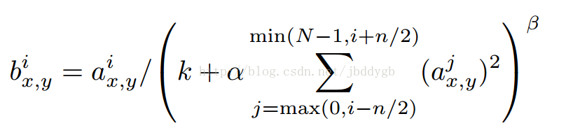
where the sum runs over n “adjacent” kernelmaps at the same spatial position, and N is the total number of kernels in thelayer. The ordering of the kernel maps is of course arbitrary and determined beforetraining begins. This sort of response normalization implements a form oflateral inhibition inspired by the type found in real neurons, creatingcompetition for big activities amongst neuron outputs computed using differentkernels. The constants k; n; α, and β are hyper-parameters whose values aredetermined using a validation set; we used k = 2, n = 5, α = 10−4, and β =0:75.
33.3 局部响应归一化
Relus单元有个很振奋人心的特点就是它们不需要输入是归一化的,不会饱和。如果至少一些训练样本产生了一个正的输入到relu单元,学习过程会发生在这个神经元上。然而我们任然发现,接下来的局部归一化有助于泛华。其中会对n个临近的在同一个位置的滤波结果进行相加,N是这一层所有滤波器的总数,滤波器的顺序当然是在开始的时候就决定的,这种响应归一化顺序实现了一种侧向压抑,为不同的滤波器之间创造一种竞争机制,其中的恒定变量,k。n。α, and β是超参数,是通过验证集确定。我们使用 k = 2, n = 5, α = 10−4, and β = 0:75.
We applied this normalization afterapplying the ReLU nonlinearity in certain layers (see Section 3.5). This schemebears some resemblance to the local contrast normalization scheme of Jarrett etal. [11], but ours would be more correctly termed “brightness normalization”,since we do not subtract the mean activity. Response normalization reduces ourtop-1 and top-5 error rates by 1.4% and 1.2%, respectively. We also verifiedthe effectiveness of this scheme on the CIFAR-10 dataset: a four-layer CNNachieved a 13% test error rate without normalization and 11% withnormalization3.
我们将这种归一化技术用在Relu单元之后,参看3.5。这种方法可以类似一些局部反向归一化,但是我们的会更正确亲相遇“亮度归一化”,因为我们不会提取平均灰度值,响应归一化分别减少了我们的top1和top5准确率1.4%和1.2%。我们还证明了这种方法在CIFAR-10上很高效,一个四层的CNN不归一化取得了13%的错误率,归一化后取得11%错误率。
3.4 Overlapping Pooling
Pooling layers in CNNs summarize theoutputs of neighboring groups of neurons in the same kernel map. Traditionally,the neighborhoods summarized by adjacent pooling units do not overlap (e.g., [17,11, 4]). To be more precise, a pooling layer can be thought of as consisting ofa grid of pooling units spaced s pixels apart, each summarizing a neighborhoodof size z × z centered at the location of the pooling unit. If we set s = z, weobtain traditional local pooling as commonly employed in CNNs. If we set s <z, we obtain overlapping pooling. This is what we use throughout our network,with s = 2 and z = 3. This scheme reduces the top-1 and top-5 error rates by0.4% and 0.3%, respectively, as compared with the non-overlapping scheme s = 2;z = 2, which produces output of equivalent dimensions. We generally observeduring training that models with overlapping pooling find it slightly moredifficult to overfit.
3.4 重叠池化
池化层在CNN中会简化在同一滤波器卷积后的输出结果,一般的,邻居不领域的池化单元不会重叠,说的更精准:一个池化层可以认为是有一个池化网格单元组成的,从而把s个像素点分开每个池化窗口从坐标周围z*z的窗口中提取,如果我们使得s=z,那么就和传统的CNN网络一样了,如果我们让s<z,那么我们就获得了重叠池化,我们现在的网络就是这么使用的。我们从整体上观察整个训练过程,使用overlaping的网络会更难发生过拟合
3.5 Overall Architecture
Now we are ready to describe the overallarchitecture of our CNN. As depicted in Figure 2, the net
contains eight layers with weights; thefirst five are convolutional and the remaining three are fullyconnected. Theoutput of the last fully-connected layer is fed to a 1000-way softmax whichproduces a distribution over the 1000 class labels. Our network maximizes themultinomial logistic regression objective, which is equivalent to maximizingthe average across training cases of the log-probability of the correct labelunder the prediction distribution.
3.5 整体框架
现在我们以及准备好对整体框架进行梳理描述了,如图2所示,这个网络包含8个参数层,5个全卷积和3个全连接,最后的全卷积输出会放入1000维的softmax层中,产生1000个类别分布,我们的网络最大化了多维正太逻辑回归的目的,相当于最大化训练样例在预测准确类别分布时的log概率的平均值。
The kernels of the second, fourth, andfifth convolutional layers are connected only to those kernel maps in theprevious layer which reside on the same GPU (see Figure 2). The kernels of thethird convolutional layer are connected to all kernel maps in the second layer.The neurons in the fullyconnected layers are connected to all neurons in theprevious layer. Response-normalization layers follow the first and secondconvolutional layers. Max-pooling layers, of the kind described in Section 3.4,follow both response-normalization layers as well as the fifth convolutionallayer. The ReLU non-linearity is applied to the output of every convolutionaland fully-connected layer. The first convolutional layer filters the 224×224×3input image with 96 kernels of size 11×11×3 with a stride of 4 pixels (this isthe distance between the receptive field centers of neighboring 3We cannotdescribe this network in detail due to space constraints, but it is specifiedprecisely by the code and parameter files provided here:http://code.google.com/p/cuda-convnet/.
第二个,第四个和第五个卷积层滤波器都是和前一层上的同一个GPU的滤波结果相连接(如图2)。第三个卷积层则是和所有的滤波结果相连接全连接的层上是和上一层所有的神经元相连接的。响应归一化操作层会在第一个和第二个卷积层之后进行,最大池化层,在3.4描述的那样,是跟随在响应归一化层和第五的卷积层之后的。Relu单元则是每一个卷积和全连接输出层之后都有,第一个卷积层滤波器不224*224*3的输入图像,使用96个滤波模板,变成了11*11*3的结构,布长4个像素(这是感官上两个滤波中心的距离)。由于篇幅限制我们不能详细描述网络了,但这个在代码和权重文件中会很详细,可以看这个http://code.google.com/p/cuda-convnet/
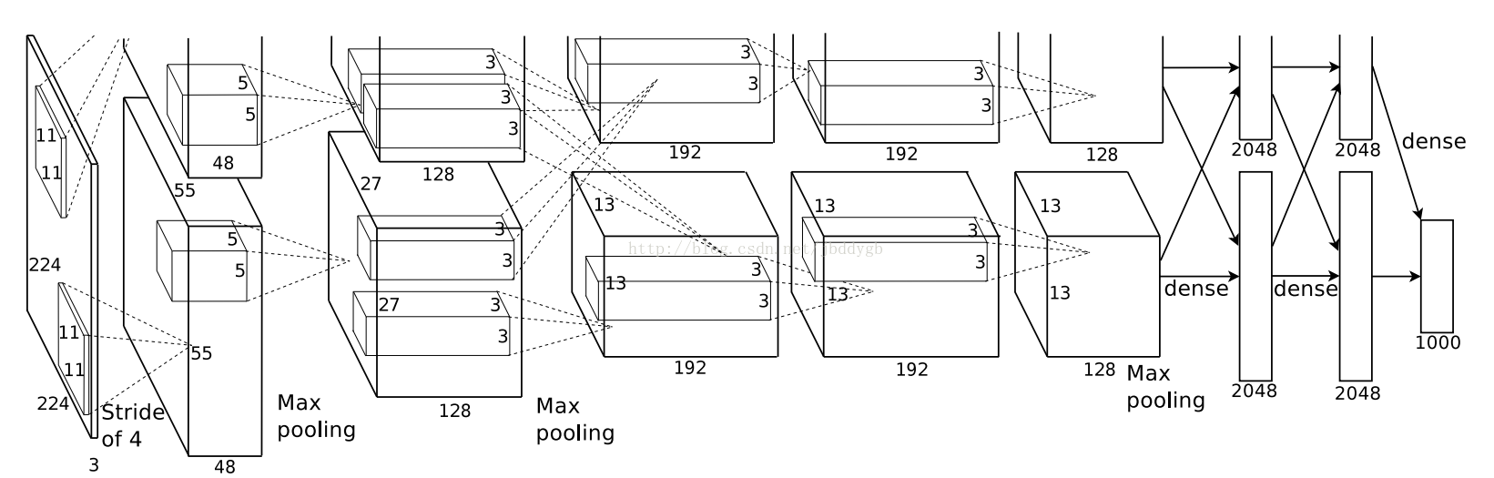
Figure 2: An illustration of thearchitecture of our CNN, explicitly showing the delineation of responsibilitiesbetween the two GPUs. One GPU runs the layer-parts at the top of the figurewhile the other runs the layer-parts at the bottom. The GPUs communicate onlyat certain layers. The network’s input is 150,528-dimensional, and the numberof neurons in the network’s remaining layers is given by253,440–186,624–64,896–64,896–43,264–4096–4096–1000.
图2.一个我们网络的架构图,清楚地可以看到两个GPU的分工,一个GPU负责上边的层,另一个负责下面,GPU通信只在特定的层进行,网络的输入是一个150*528唯独的,然后神经网络保留层的神经元数目则是 253, 440*186,624*64,896*64,896*43,264-4096-4096-1000神经元
neurons in a kernel map). The secondconvolutional layer takes as input the (response-normalized
and pooled) output of the firstconvolutional layer and filters it with 256 kernels of size 5 × 5 × 48.
The third, fourth, and fifth convolutionallayers are connected to one another without any intervening pooling ornormalization layers. The third convolutional layer has 384 kernels of size 3 ×3 × 256 connected to the (normalized, pooled) outputs of the secondconvolutional layer. The fourth convolutional layer has 384 kernels of size 3 ×3 × 192 , and the fifth convolutional layer has 256 kernels of size 3 × 3 ×192. The fully-connected layers have 4096 neurons each.
第二个卷积层作为响应归一化层的输入,第一个卷积层的输出,使用了256个卷积核,大小为5*5*46第三第四和第五个卷积层都是连接到前一个,而没有池化和归一化层。第三个卷积层有384个滤波核,大小3*3*256,适合归一化层和pooling层相连的(第二层输出作处理),第四格卷积层有384个3*3*192的滤波核,第五个256个有3*3*193的滤波核。全连接的每层有4096个神经元
4 Reducing Overfitting
Our neural network architecture has 60million parameters. Although the 1000 classes of ILSVRC
make each training example impose 10 bitsof constraint on the mapping from image to label, this
turns out to be insufficient to learn somany parameters without considerable overfitting. Below, we describe the twoprimary ways in which we combat overfitting.
4 减少过拟合
我们的神经网络结构有60000000参数,尽管是在1000个类别上的结果,每个训练样本都有10 bit的参数量,从分析都标签,学习这么多参数却不考虑过拟合是不可能的,下面我们就描述了两个简单方法组合起来防止过拟合。
4.1 Data Augmentation
The easiest and most common method toreduce overfitting on image data is to artificially enlarge the dataset usinglabel-preserving transformations (e.g., [25, 4, 5]). We employ two distinctforms of data augmentation, both of which allow transformed images to beproduced from the original images with very little computation, so thetransformed images do not need to be stored on disk. In our implementation, thetransformed images are generated in Python code on the CPU while the GPU istraining on the previous batch of images. So these data augmentation schemesare, in effect, computationally free. The first form of data augmentationconsists of generating image translations and horizontal reflections. We dothis by extracting random 224 × 224 patches (and their horizontal reflections)from the 256×256 images and training our network on these extracted patches4.This increases the size of our training set by a factor of 2048, though theresulting training examples are, of course, highly interdependent. Without thisscheme, our network suffers from substantial overfitting, which would have forcedus to use much smaller networks. At test time, the network makes a predictionby extracting five 224 × 224 patches (the four corner patches and the centerpatch) as well as their horizontal reflections (hence ten patches in all), andaveraging the predictions made by the network’s softmax layer on the tenpatches.
4.1数据增强
最简单常用的防止过拟合方法就是把图像变形,从而扩大数据集,只需要简单计算就可以,变形后图像不需要存储。直接用python函数CPU上就可以实现,而GPU训练可以同时进行,两者互不影响。第一种变形是平移和水平翻转,我们从256*256的原图中提取224*224的平移后的和翻转的图像块,这会使得我们的训练集扩大2048倍,尽管这样训练数据集之间会有很强关联性,但如果不这样,我们的网络就会持续地过拟合,这就不得不减小网络规模了。检测时,网络从原图提取五个区域(四个角和中间部分)224*224的块,另外就是水平翻转,这样总共10种变化,最后的测试结果是10个块的平均softmax输出。
The second form of data augmentationconsists of altering the intensities of the RGB channels in training images.Specifically, we perform PCA on the set of RGB pixel values throughout the ImageNettraining set. To each training image, we add multiples of the found principalcomponents, 4This is the reason why the input images in Figure 2 are 224 × 224× 3-dimensional. 5with magnitudes proportional to the corresponding eigenvaluestimes a random variable drawn from a Gaussian with mean zero and standard deviation0.1. Therefore to each RGB image pixel we add the following quantity:
where pi and λi are ith eigenvector andeigenvalue of the 3 × 3 covariance matrix of RGB pixel values, respectively,and αi is the aforementioned random variabl. Each αi is drawn only once for allthe pixels of a particular training image until that image is used for trainingagain, at which point it is re-drawn. This scheme approximately captures animportant property of natural images, namely, that object identity is invariantto changes in the intensity and color of the illumination. This scheme reducesthe top-1 error rate by over 1%.
第二个数据增强的方法是改变RGB通道的强度,特别的,我们使用PCA对Imagenet训练集合RGB数据进行操作,对每隔训练图像,我们都乘以主成分(还没太理解PCA的作用),这是也就是为什么我们的输入图像在图2中是224*224*3,将每个特征值的成份量乘以一个随机高斯系数(均值0,反差0.1),因此,每隔RGB图像像素 ,我们使用下面的量
pi 和 λi 是3*3的特征向量和特征值, 来自RGB数据的 3 × 3 的协方差矩阵。 αi 是之前提到的随机变量,每个 αi 都只提取一次,直到这幅图像再次用作训练,在每个点都重新提取,这个方法大概是为了提取自然图像的重要特征。也就是说,对象属性在亮度和颜色变化过程中是保持不变的。这个可以减少约1%的错误率
4.2 Dropout
Combining the predictions of many differentmodels is a very successful way to reduce test errors [1, 3], but it appears tobe too expensive for big neural networks that already take several days totrain. There is, however, a very efficient version of model combination thatonly costs about a factor of two during training. The recently-introducedtechnique, called “drpout” [10], consists of setting to zero the output of eachhidden neuron with probability 0.5. The neurons which are“dropped out”in this way do not contribute to the forward pass and do not participate inbackpropagation.
4.2 dropout
组合各种模型结果是一种很好的减少测试错误率的方法,但是对于神经网络,这却是很耗时的,最高效的组合方式也要花两倍的时间,最近提出一种叫“dropout”的技术,是通过50%的机率把每个隐藏神经元的输出变为0,这样,神经元相当于被抛弃了,对于前项传播就没有任何影响,也不会参与反向传播
So every time an input is presented, theneural network samples a different architecture, but all these architecturesshare weights. This technique reduces complex co-adaptations of neurons, sincea neuron cannot rely on the presence of particular other neurons. It is,therefore, forced to learn more robust features that are useful in conjunctionwith many different random subsets of the other neurons. At test time, we useall the neurons but multiply their outputs by 0.5, which is a reasonableapproximation to taking the geometric mean of the predictive distributionsproduced by the exponentially-many dropout networks. We use dropout in thefirst two fully-connected layers of Figure 2.
因此每一次输入,神经网络都会建立不同的结构,但是所有这些结构共享权重,这个技术减少了复杂的神经网络组合,因为一个神经元可以依赖于特定的神经元输入。因此我们能学习到很对针对不同情况下子集的特征表达,在测试时候,我们使用所有的神经元,但是把他们的输出乘以0.5,这是一种将几何上概率上平均组合各种网络结构的方法,我们在前两个全连接层使用dropout,如图2所示。
Without dropout, our network exhibitssubstantial overfitting. Dropout roughly doubles the number of iterationsrequired to converge.
没有dropout 我们的网络架构就会表现出持续的过拟合,dropout粗略上看,使得网络收敛的迭代次数翻倍了。
5 Details of learning
We trained our models using stochasticgradient descent with a batch size of 128 examples, momentum of 0.9, and weightdecay of 0.0005. We found that this small amount of weight decay was importantfor the model to learn. In other words, weight decay here is not merely aregularizer: it reduces the model’s training error. The update rule for weightw was:
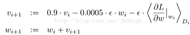
where i is the iteration index, v is themomentum variable, is the learning rate,and 
5实现细节
我们使用随机梯度下降法来训练模型,一次性使用批量128个样本,惯性势能参数momentumm 0.9梯度调整步长0.0005.我们发现,这个很小的数量的梯度步长对于模型训练是很重要的,换句话说,权重调整步长不仅仅是一个约束量,它还影响到模型的训练错误率。w的更新准则为:
其中i是迭代标签,v是惯性参数,Si是学习速率, 是平均第i个批量两本Di的关于w偏导数平均值。我们在每一层使用了0均值-0.01方差的高斯分布来作为初始化权重,我们初始化神经元偏差,在第2层,第4层,第5层卷积层,在全连接层也是如此,恒定量1,这个初始化加速了早=先前的学习,提供Relu单元正数输入,我们初始化神经元偏差,在其余的层数设置为0,我们使用相等的学习速率对所有的层进行学习。在训练过程中人为地调节,启发是,我们把学习速率除以10,当验证错误率不再改变的时候,这样学习速率定为 0.01 并且终止之前会减少三次。我们训练了神经网络大约90次循环,在120万张图像上花费了5-6天,Nvidia GTX580 3GB GPUs。
6 Results
Our results on ILSVRC-2010 are summarizedin Table 1. Our network achieves top-1 and top-5 test set error rates of 37.5%and 17.0%5. The best performance achieved during the ILSVRC-2010 competitionwas 47.1% and 28.2% with an approach that averages the predictions produced fromsix sparse-coding models trained on different features [2], and since then thebest published results are 45.7% and 25.7% with an approach that averages the predictionsof two classifiers trained on Fisher Vectors (FVs) computed from two types ofdensely-sampled features [24].
6 结果
Table对结果进行了总结,我们的网络获得了top137.5%准确率和top5 17.0%准确率,之前最好的表现是在ISLVRC2010 上取得的 47.1%,和 28.2%,该方法是利用不通特征建立的六个稀疏编码的模型,直到该文章发表,最好的准确率是45.7%和25.7%,使用了两个分类器的组合,使用了两种稠密特征上提取的费舍尔向量
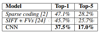
Table1: Comparison of results on ILSVRC-
2010test set. In italics are best results
表1ILSVRC-2010上的结果比较,加粗的是最好的
achieved by others. We also entered ourmodel in the ILSVRC-2012 competition and report our results in Table 2. Sincethe ILSVRC-2012 test set labels are not publicly available, we cannot reporttest error rates for all the models that we tried. In the remainder of thisparagraph, we use validation and test error rates interchangeably because inour experience they do not differ by more than 0.1% (see Table 2).
我们还在ILSVRC-2012上进行了我们模型测试,结果在Table2,由于ILSVRC-2012测试标签是不可获取的我们不能。把其他模型的结果放上来。这一章节的剩余部分,我们使用验证集来测试错误率的变化,因为在我们的经验中,他们不会变化超过0.1%
The CNN described in this paper achieves atop-5 error rate of 18.2%. Averaging the predictions of five similar CNNs givesan error rate of 16.4%. Training one CNN, with an extra sixth convolutionallayer over the last pooling layer, to classify the entire ImageNet Fall 2011release (15M images, 22K categories), and then “fine-tuning” it on ILSVRC-2012gives an error rate of 16.6%. Averaging the predictions of two CNNs that werepre-trained on the entire Fall 2011 release with the aforementioned five CNNsgives an error rate of 15.3%. The second-best contest entry achieved an errorrate of 26.2% with an approach that averages the predictions of severalclassifiers trained on FVs computed from different types of densely-sampledfeatures [7].
这篇文章提到的CNN模型的top-5准确率是18.2%。另外还有5个类似的模型达到平均16.4%的准确率。训练一个CNN模型,包含另外6个卷积层,在池化之后,来分类整个Imagenet
然后有效调节它可以获得准确率“16.6%”平均计算两个在2011数据集上训练的CNN,错误率是15.3%,而第二名的错误率是26.2% 使用了两个分类器的组合,使用了两种稠密特征上提取的费舍尔向量。
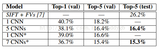
Table 2: Comparison of error rates onILSVRC-2012 validation and test sets. In italics are best results achieved byothers. Models with an asterisk* were “pre-trained” to classify the entireImageNet 2011 Fall release. See Section 6 for details.
图2:ILSVRC-2012 验证集合和测试集上的错误率结果,其中加粗的是其他人获取最好的结果。模型名字加上*好的是预先训练的用于分类整个Imagenet-2011数据集的,详细请看第六节。
Finally, we also report our error rates onthe Fall 2009 version of ImageNet with 10,184 categories and 8.9 millionimages. On this dataset we follow the convention in the literature of usinghalf of the images for training and half for testing. Since there is noestablished test set, our split necessarily differs from the splits used byprevious authors, but this does not affect the results appreciably. Our top-1and top-5 error rates on this dataset are 67.4% and 40.9%, attained by the netdescribed above but with an additional, sixth convolutional layer over the lastpooling layer. The best published results on this dataset are 78.1% and 60.9%[19].
最后,我们还给出了离线数据集Imagenet2009上的结果,包含了10184分种类。890万张图像。在这个数据集上,我们使用一半作为训练,一半作为测试。由于没有公开的测试数据集。我们的分割的方法和之前不太一样,但是这不影响最后结果。我们的top-1 和top-5错误率是67.4%和40.9%。使用了后面添加6个卷积层的方法,最好的结果是78.1%和60.9%
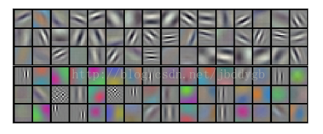
Figure 3 shows the convolutional kernelslearned by the network’s two data-connected layers. The network has learned avariety of frequency- and orientation-selective kernels, as well as variouscolored blobs. Notice the specialization exhibited by the two GPUs, a result ofthe restricted connectivity described in Section 3.5. The kernels on GPU 1 arelargely color-agnostic, while the kernels
Figure 3: 96 convolutional kernels of size 11×11×3learned by the first convolutional layer on the 224×224×3 inputimages. The top 48 kernels were learned on GPU 1 while the bottom 48 kernelswere learned on GPU 2. See Section 6.1 for details.
图3,96个11*11*3的卷积模版,通过第一个卷积层224*224*3的图像学习到的,前48个卷积模版是在GPU1上学习得到的,而后48个是在GPU2上学习。细节请看6.1节。
6.1 Qualitative Evaluations
Figure 3 shows the convolutional kernelslearned by the network’s two data-connected layers. The
network has learned a variety of frequency-and orientation-selective kernels, as well as various colored blobs. Notice thespecialization exhibited by the two GPUs, a result of the restrictedconnectivity described in Section 3.5. The kernels on GPU 1 are largelycolor-agnostic, while the kernels on GPU 2 are largely color-specific. Thiskind of specialization occurs during every run and is independent of anyparticular random weight initialization (modulo a renumbering of the GPUs).
5The error rates without averagingpredictions over ten patches as described in Section 4.1 are 39.0% and 18.3%.
6.1 定量分析
图3展示了神经网络中数据连接层卷积模版的学习。神经网络学习到了多种多样的频率方向滤波器,还有许多颜色块,注意到特殊情况在两个GPU上,GPU1上的都是颜色不敏感的,而GPU2上的都是颜色敏感的,这种结果在每次训练时都会发生,不论任何初始化权重都会这样,平均错误率时39。0%和18.3%。
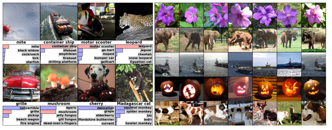
Figure 4: (Left) Eight ILSVRC-2010 test images and the five labels consideredmost probable by our model. The correct label is written under each image, andthe probability assigned to the correct label is also shown with a red bar (ifit happens to be in the top 5). (Right) Five ILSVRC-2010 test images in thefirst column. The remaining columns show the six training images that producefeature vectors in the last hidden layer with the smallest Euclidean distancefrom the feature vector for the test image.
图4:(左)8个ISLVRC-2012的测试图像和五个我们的模型给出的坐标,准确的坐标写在图像下方,概率也以红色条形图表示了出来(如果前五里面有预测准确的话)。(右)第一列是5个ISLVRC-2012的测试图像。剩下的列表示6个产生出和测试图像特征欧氏距离最接近的训练图像。
In the left panel of Figure 4 wequalitatively assess what the network has learned by computing its top-5predictions on eight test images. Notice that even off-center objects, such asthe mite in the top-left, can be recognized by the net. Most of the top-5 labelsappear reasonable. For example, only other types of cat are consideredplausible labels for the leopard. In some cases (grille, cherry) there isgenuine ambiguity about the intended focus of the photograph.
Another way to probe the network’s visual knowledgeis to consider the feature activations induced by an image at the last,4096-dimensional hidden layer. If two images produce feature activation vectorswith a small Euclidean separation, we can say that the higher levels of theneural network consider them to be similar. Figure 4 shows five images from thetest set and the six images from the training set that are most similar to eachof them according to this measure. Notice that at the pixel level, theretrieved training images are generally not close in L2 to the query images inthe first column. For example, the retrieved dogs and elephants appear in avariety of poses. We present the results for many more test images in thesupplementary material. Computing similarity by using Euclidean distancebetween two 4096-dimensional, real-valued vectors is inefficient, but it couldbe made efficient by training an auto-encoder to compress these vectors toshort binary codes. This should produce a much better image retrieval methodthan applying autoencoders to the raw pixels [14], which does not make use ofimage labels and hence has a tendency to retrieve images with similar patternsof edges, whether or not they are semantically similar.
7 Discussion
Our results show that a large, deepconvolutional neural network is capable of achieving recordbreaking results ona highly challenging dataset using purely supervised learning. It is notable thatour network’s performance degrades if a single convolutional layer is removed.For example, removing any of the middle layers results in a loss of about 2%for the top-1 performance of the network. So the depth really is important forachieving our results. To simplify our experiments, we did not use anyunsupervised pre-training even though we expect that it will help, especiallyif we obtain enough computational power to significantly increase the size ofthe network without obtaining a corresponding increase in the amount of labeleddata. Thus far, our results have improved as we have made our network largerand trained it longer but we still have many orders of magnitude to go in orderto match the infero-temporal pathway of the human visual system. Ultimately wewould like to use very large and deep convolutional nets on video sequenceswhere the temporal structure provides very helpful information that is missingor far less obvious in static images.


 6159
6159


 被折叠的 条评论
为什么被折叠?
被折叠的 条评论
为什么被折叠?
 到【灌水乐园】发言


