Coursera | Andrew Ng (01-week-2-2.14)—向量化 logistic 回归的梯度输出

该系列仅在原课程基础上部分知识点添加个人学习笔记，或相关推导补充等。如有错误，还请批评指教。在学习了 Andrew Ng 课程的基础上，为了更方便的查阅复习，将其整理成文字。因本人一直在学习英语，所以该系列以英文为主，同时也建议读者以英文为主，中文辅助，以便后期进阶时，为学习相关领域的学术论文做铺垫。- ZJ

Coursera 课程 |deeplearning.ai |网易云课堂

---

转载请注明作者和出处：ZJ 微信公众号-「SelfImprovementLab」

知乎：https://zhuanlan.zhihu.com/c_147249273

CSDN：http://blog.csdn.net/JUNJUN_ZHAO/article/details/78948859

---

2.14 Vectorizing Logistic Regression’s Gradient Computation

向量化 logistic 回归的梯度输出

(字幕来源：网易云课堂)

In the previous video,you saw how you can use vectorization to compute their predictions,the lowercase a’s for an entire training set all at the same time.In this video, you see how you can use vectorization to also perform the gradient computations for all m training samples.Again, all those at the same time.And then at the end of this video,we’ll put it all together and show how you can derive a very efficient implementation of logistic regression.

在之前的视频中，你知道了如何通过向量化同时计算整个训练集预测值 a。在这个视频中你将学会如何向量化，计算 m 个训练数据的梯度，强调一下是同时计算，在本视频的末尾，我们会将之前讲的结合起来 向你展示，如何得到一个非常高效的 logistic 回归的实现。

So, you may remember that for the gradient computation,what we did was we computed $dz^{(1)}$ for the first example,which could be $a^{(1)}$ minus $y^{(1)}$ and then $dz^{(2)}$ equals $a^{(2)}$ minus $y^{(2)}$ and so on.And so on for all m training examples.So, what we’re going to do is define a new variable,dZ is going to be $dz^{(1)}$, $dz^{(2)}$, $dz^{(m)}$.Again, all the d lowercase z variables stacked horizontally.So, this would be 1 by m matrix or alternatively a m dimensional row vector.Now recall that from the previous slide,we’d already figured out how to compute capital A which was this:$a^{(1)}$ through $a^{(m)}$ and we had defined capital $Y$ as $y^{(1)}$ through $y^{(m)}$.Also you know, stacked horizontally.

你可能记得讲梯度计算时，我列举了几个例子，$dz^{(1)} = a^{(1)}-y^{(1)}$，$dz^{(2)}=a^{(2)}-y^{(2)}$等等列举下去，对 $m$ 个训练数据做同样的运算，我们现在可以定义一个新的变量，$dZ = [dz^{(1)},dz^{(2)},...dz^{(m)}]$，所有的 $dz$ 变量横向排列，$dZ$ 将会是一个$1*m$ 的矩阵，或者说一个 $m$ 维行向量，回忆之前的幻灯片，我们已经描述了如何计算 $A$,即$[a^{(1)},...a^{(m)}]$，我们已经定义了大写字母$Y=[y^{(1)},...y^{(m)}]$，像之前一样$y^{(1)},...y^{(m)}$横向排列。

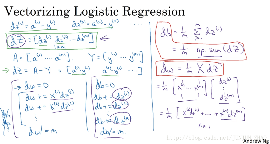
So, based on these definitions,maybe you can see for yourself that $dZ$ can be computed as just A minus Y because it’s going to be equal to $a^{(1)} - y^{(1)}$. So, the first element, $a^{(2)} - y^{(2)}$,so in the second element and so on.And, so this first element $a^{(1)} - y^{(1)}$ is exactly the definition of $dz^{(1)}$.The second element is exactly the definition of $dz^{(2)}$ and so on.So, with just one line of code,you can compute all of this at the same time.Now, in the previous implementation,we’ve gotten rid of one for loop already but we still had this second for loop over training examples.So we initialize $dw$ to zero to a vector of zeroes.But then we still have to loop over training examples where we have dw plus equals $x^{(1)}$ times $dz^{(1)}$,for the first training example dw plus equals $x^{(2)} ，dz^{(2)}$ and so on.

基于这些定义，你也许会发现我们可以这样计算$dZ$，$dZ = A-Y$ 这等于，$[a^{(1)}-y^{(1)},a^{(2)}-y^{(2)}...]$，以此类推，第一个元素$a^{(1)}-y^{(1)}$就是$dz^{(1)}$，第二个元素就是$dz^{(2)}$ …，所以仅需要一行代码，你就可以同时完成这所有的计算，在之前的实现中，我们已经去掉了一个 for 循环 但是，我们仍然有一个遍历训练集的循环，我们使用$dw=0$将$dw$初始化为 0 向量，但是我们还有一个遍历训练集的循环，对第一个训练样本有$dw+=x^{(1)}*dz^{(1)}$，第二个样本$dw+=x^{(2)}*dz^{(2)}$ …

So we do the m times and then dw divide equals by m and similarly for b, right?db was initialized as 0 and db plus equals $dz^{(1)}$.db plus equals $dz^{(2)}$ down to you know $dz^{(m)}$ and db divide equals m.So that’s what we had in the previous implementation.We’d already got rid of one for loop.So, at least now dw is a vector and we went separately updating dw1,dw2 and so on.So, we got rid of that already but we still had the for loop over the M examples in the training set.So, let’s take these operations and vectorize them. Here’s what we can do, for the vectorize implementation of db was doing is basically summing up,all of these dzs and then dividing by m.

我们重复 m 次，然后 $dw/=m$ b也类似，$db$ 被初始化为 0 向量 然后 $db+=dz^{(1)}$，$db+=dz^{(2)}$ 这样重复到，$dz^{(m)}$ 接着 $db/=m$，这就是我们在之前的实现中做的，我们已经去掉了一个 for 循环，至少现在 $dw$ 是个向量了 然后我们分别，更新 $dw^{(1)} dw^{(2)}$等，我们去掉了一个 for 循环，但是还有个 for 循环遍历训练集，让我们继续下面的操作把它们向量化，我们可以这么做，向量化的实现 $db$ 只需要对，这些 $dz$ 求和 然后除以 m。

So, db is basically one over m, sum from I equals once through m of dzi and well all the dzs are in that row vector and so in Python,what you do is implement you know, 1 over m times np. sum of the Z.So, you just take this variable and call the np.sum function on it and that would give you db.How about dw or just write out the correct equations who can verify is the right thing to do.Dw turns out to be one over m, times the matrix X times dZ transpose.And, so kind of see why that’s the case.This equal to one over m then the matrix X’s,x^{(1)} through x^{(m)} stacked up in columns like that and dZ transpose is going to be $dz^{(1)}$ down to $dz^{(m)}$ like so.

而 $db=1/m$，对$dz^{(1)}$到$dz^{(m)}$求和，所有的$dz$组成了一个行向量 所以，在 Python 中你仅需要 ，1/m*np.sum(dZ)，你只要把这个变量传给np.sum函数，就可以得到$db$，那么$dw$呢? 先写出正确的公式，这才能证明我们做的是正确的，dw=1/m*X*dZ转置，让我们看看为什么是这样，这等于$1/m$乘以，列向量$x^{(1)}...x^{(m)}$堆叠起来，$dZ$转置是$dz^{(1)}$…$dz^{(m)}$

And so, if you figure out what this matrix times this vector works out to be,it is turns out to be one over m times x^{(1)} $dz^{(1)}$ plus… plus x^{(m)} $dz^{(m)}$.And so, this is a n*1 vector and this is what you actually end up with,with dw because dw was taking these you know, xi dzi and adding them up and so that’s what exactly this matrix vector multiplication is doing and so again,with one line of code you can compute dw.So, the vectorized implementation of the derivative calculations is just this,you use this line to implement db and use this line to implement dw and notice that without the for loop over the training set,you can now compute the updates you want to your parameters.

如果你明白这个矩阵，乘以这个向量会得到什么，这等于$1/m$，这等于 $1/m*[x^{(1)}*dz^{(1)}+...+x^{(m)}*dz^{(m)}]$，这是一个$n×1$的向量，也就是你最终得到的，因为$dw$中包括了这些，$x_i*dz_i$ 然后把它们加起来，就是这个矩阵和向量相乘做的，只要一行代码你就可以计算出$dw$，向量化计算导数的实现，就像下面这样，你用这行代码计算$db$ 这行代码计算$dw$，注意我们没有在训练集上使用 for 循环，现在你可以计算参数的更新。

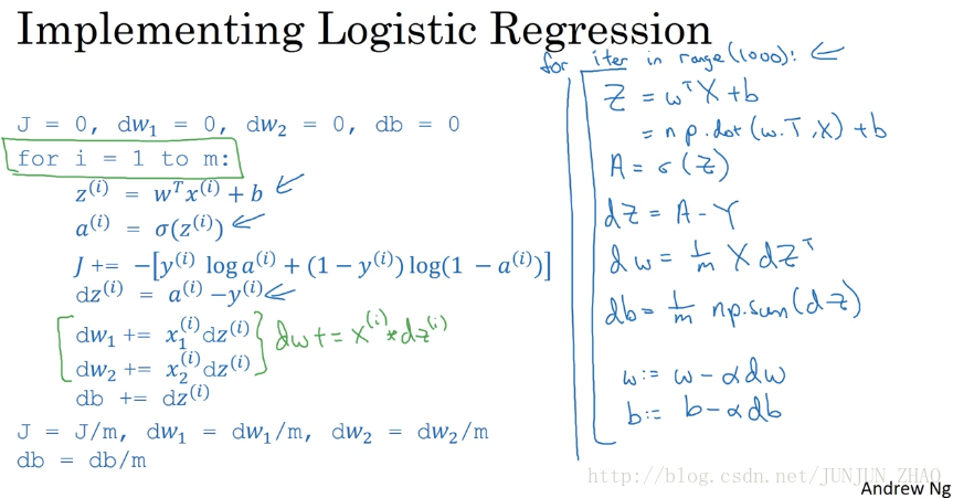
So now, let’s put all together into how you would actually implement logistic regression.So, this is our original,highly inefficient non vectorize implementation.So, the first thing we’ve done in the previous video was get rid of this volume, right?So, instead of looping over dw1, dw2 and so on,we have replaced this with a vector value dw which is dw+= xi,which is now a vector times dz(i).But now, we will see that we can also get rid of not just for loop of those but also get rid of this for loop.So, here is how you do it.So, using what we have from the previous slides,you would say, capitalZ, Z equal to w transpose X + b and the code you is write capital Z equals np. w transpose X + b and then A equals sigmoid of capital Z.

现在 我们回顾之前所学，看看应该如何实现一个 logistic 回归，这是我们之前的，没有向量化非常低效，首先是我们在前一个视频中，做的去掉这一堆，不用循环遍历 $dw1 dw2$等，我们已经用一个向量化的代码$dw+=x^{(i)}$替换这些，$x^{(i)}$是一个向量 给它乘以$dz^{(i)}$，现在 我们不仅要取消那些循环，还要取消掉这个 for 循环，你可以这么做，用前面幻灯片我们得到的，$Z=w^TX + B$，你的代码 应该是Z=np.dot(w.T,X)+b，然后A = sigmoid(Z)。

So, you have now computed all of this and all of this for all the values of I.Next on the previous slide,we said you would compute dZ equals A - Y.So, now you computed all of this for all the values of i.Then, finally dw equals 1/m x dZ transpose and db equals 1/m of you know, np. db=1/m np.sum(dZ) So, you’ve just done front propagation and back propagation,really computing the predictions and computing the derivatives on all M training examples without using a for loop.And so the gradient descent update then would be you know w gets updated as w minus the learning rate times dw which was just computed above and b is update as b minus the learning rate times db.

你已经对所有 i，完成了这些和这些计算，之前的幻灯片，我们知道你还应该计算$dZ=A-Y$，就对所有 i 完成了这个计算，最后 dw=1/m XdZ.T，db=1/m np.sum(dZ)，你完成了正向和反向传播，确实实现 对所有训练样本进行预测和求导，而且没有使用一个 for 循环，然后梯度下降更新参数，w=w-α*dw 其中 α 是学习率，b 等于b-α*db 其中 α 是学习率。

dZ，dw，db 的求导/梯度

Z = np.dot(w.T,X) + b
A = sigmoid(Z)
dZ = A-Y
dw = 1/m*np.dot(X,dZ.T)
db = 1/m*np.sum(dZ)

w = w - alpha*dw
b = b - alpha*db

Sometimes it’s pretty close to notice that it is an assignment,but I guess I haven’t been totally consistent with that notation.But with this, you have just implemented a single iteration of gradient descent for logistic regression.Now, I know I said that we should get rid of explicit for loops whenever you can but if you want to implement multiple iteration as a gradient descent then you still need a for loop over the number of iterations.So, if you want to have a thousand deliveration of gradient descent,you might still need a for loop over the iteration number.There is an outermost for loop like that then I don’t think there is any way to get rid of that for loop.

有时候应该用这个赋值符号，不过我对这个符号的使用前后可能不一，有了这些，我们就实现了 logistic 回归的梯度下降一次迭代，我说过我们应该尽量不用显式 for 循环，尽量不要用，但如果你，如果你希望多次迭代进行，梯度下降 那么你仍然需要 fo r循环，如果你要求1000次导数进行梯度下降，你或许仍旧需要一个 for 循环，这个最外面的 for 循环，我认为应该没有方式把它去掉。

But I do think it’s incredibly cool that you can implement at least one iteration of gradient descent without needing to use a full loop.So, that’s it you now have a highly vectorize and highly efficient implementation of gradient descent for logistic regression. There is just one more detail that I want to talk about in the next video, which is in our description here.I briefly alluded to this technique called broadcasting.Broadcasting turns out to be a technique that Python and numpy allows you to use to make certain parts of your code also much more efficient.So, let’s see some more details of broadcasting in the next video.

不过我觉得实现了一次梯度下降迭代，而不需要任何 for 循环还是很爽的，你得到了一个高度向量化的，非常高效的 logistic 回归的梯度下降法，这里有一些细节 我想在下个视频中讨论，这里我简单提一下，这种技术被称为“广播”，“广播”也是一种能够使你的，Python 和 Numpy 部分代码，更高效的技术，我们在下个视频中学习关于“广播”的更多细节。

---

重点总结：

所有 m 个样本的线性输出 $Z$ 可以用矩阵表示：

$Z = w^{T}X+b$

Z = np.dot(w.T,X) + b
A = sigmoid(Z)

逻辑回归梯度下降输出向量化

• $dZ$对于$m$个样本，维度为$（1,m）$，表示为：

  $dZ = A - Y$

• db可以表示为：

$db = \dfrac{1}{m}\sum_{i=1}^{m}dz^{(i)}$

 db = 1/m * np.sum(dZ)

• dw可表示为：

$dw = \dfrac{1}{m}X\cdot dZ^{T}$

dw = 1/m*np.dot(X,dZ.T)

单次迭代梯度下降算法流程:

Z = np.dot(w.T,X) + b
A = sigmoid(Z)
dZ = A-Y
dw = 1/m*np.dot(X,dZ.T)
db = 1/m*np.sum(dZ)

w = w - alpha*dw
b = b - alpha*db

参考文献：

[1]. 大树先生.吴恩达Coursera深度学习课程 DeepLearning.ai 提炼笔记（1-2）– 神经网络基础

---

PS: 欢迎扫码关注公众号：「SelfImprovementLab」！专注「深度学习」，「机器学习」，「人工智能」。以及 「早起」，「阅读」，「运动」，「英语 」「其他」不定期建群 打卡互助活动。