


Neural Networks Learning
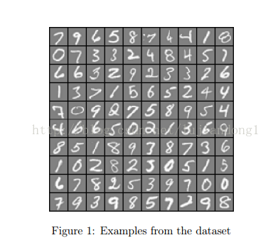
这次试用的数据和上次是一样的数据。5000个training example,每一个代表一个数字的图像,图像是20x20的灰度图,400个像素的每个位置的灰度值组成了一个training example。
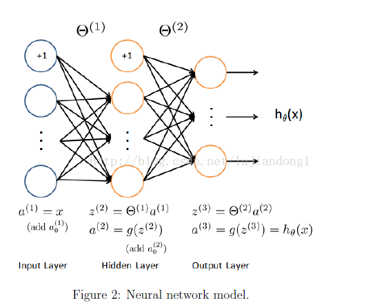
Model representation
Feedforward and cost function
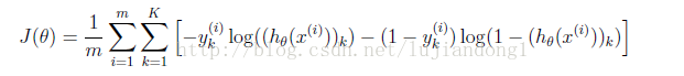
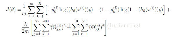
Regularized cost function
function [J grad] = nnCostFunction(nn_params, ...
input_layer_size, ...
hidden_layer_size, ...
num_labels, ...
X, y, lambda)
%NNCOSTFUNCTION Implements the neural network cost function for a two layer
%neural network which performs classification
% [J grad] = NNCOSTFUNCTON(nn_params, hidden_layer_size, num_labels, ...
% X, y, lambda) computes the cost and gradient of the neural network. The
% parameters for the neural network are "unrolled" into the vector
% nn_params and need to be converted back into the weight matrices.
%
% The returned parameter grad should be a "unrolled" vector of the
% partial derivatives of the neural network.
%
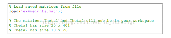
% Reshape nn_params back into the parameters Theta1 and Theta2, the weight matrices
% for our 2 layer neural network
Theta1 = reshape(nn_params(1:hidden_layer_size * (input_layer_size + 1)), ...
hidden_layer_size, (input_layer_size + 1));
Theta2 = reshape(nn_params((1 + (hidden_layer_size * (input_layer_size + 1))):end), ...
num_labels, (hidden_layer_size + 1));
% Setup some useful variables
m = size(X, 1);
% You need to return the following variables correctly
J = 0;
Theta1_grad = zeros(size(Theta1));
Theta2_grad = zeros(size(Theta2));
% ====================== YOUR CODE HERE ======================
% Instructions: You should complete the code by working through the
% following parts.
%
% Part 1: Feedforward the neural network and return the cost in the
% variable J. After implementing Part 1, you can verify that your
% cost function computation is correct by verifying the cost
% computed in ex4.m
%
% Part 2: Implement the backpropagation algorithm to compute the gradients
% Theta1_grad and Theta2_grad. You should return the partial derivatives of
% the cost function with respect to Theta1 and Theta2 in Theta1_grad and
% Theta2_grad, respectively. After implementing Part 2, you can check
% that your implementation is correct by running checkNNGradients
%
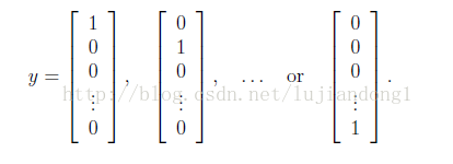
% Note: The vector y passed into the function is a vector of labels
% containing values from 1..K. You need to map this vector into a
% binary vector of 1's and 0's to be used with the neural network
% cost function.
%
% Hint: We recommend implementing backpropagation using a for-loop
% over the training examples if you are implementing it for the
% first time.
%
% Part 3: Implement regularization with the cost function and gradients.
%
% Hint: You can implement this around the code for
% backpropagation. That is, you can compute the gradients for
% the regularization separately and then add them to Theta1_grad
% and Theta2_grad from Part 2.
%
%%完全向量化版
a1 = [ones(m,1) X]; %5000*401
z2 = a1*Theta1'; %5000*25
a2 = [ones(size(z2,1),1) sigmoid(z2)]; %5000*(25+1)
z3 = a2*Theta2'; %5000*10
a3 = sigmoid(z3);
h=a3;
%-----------------Part 3: Compute Cost (Feedforward)------- -------------
Y=zeros(m,num_labels);
for i=1:num_labels
Y(:,i)=(y==i);
end
J = 1/m*sum(sum(-Y.*log(h)-(1-Y).*log(1-h)));
%--------------------------------------------------------------------------
%%正则化后
J = J + lambda/2/m*( sum(sum(Theta1(:,2:end).^2)) + sum(sum(Theta2(:,2:end).^2)) );
% compute delta
delta3=zeros(m, num_labels);
for k = 1 : num_labels
delta3(:,k) = a3(:,k) - (y==k); %5000*10
end
delta2 = delta3 * Theta2 .* [ones(size(z2,1),1) sigmoidGradient(z2)]; %5000*26
%compute Delta
Delta1 = delta2(:,2:end)' * a1; %25*401
Delta2 = delta3' * a2; %10*26
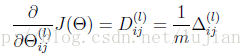
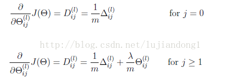
% compute Theta_grad
Theta1_grad = 1/m*Delta1;
Theta2_grad = 1/m*Delta2;
% 正则化grad
reg1 = lambda/m*Theta1;
reg2 = lambda/m*Theta2;
reg1(:,1) = 0;
reg2(:,1) = 0;
Theta1_grad = Theta1_grad + reg1;
Theta2_grad = Theta2_grad + reg2;
% -------------------------------------------------------------
% =========================================================================
% Unroll gradients
grad = [Theta1_grad(:) ; Theta2_grad(:)];
end
a1 = [ones(m,1) X]; %5000*401
z2 = a1*Theta1'; %5000*25
a2 = [ones(size(z2,1),1) sigmoid(z2)]; %5000*(25+1)
z3 = a2*Theta2'; %5000*10
a3 = sigmoid(z3);
h=a3;
%--------------------------------------------------------------------------
%%正则化后
J = J + lambda/2/m*( sum(sum(Theta1(:,2:end).^2)) + sum(sum(Theta2(:,2:end).^2)) );
---------------------------------------------------------------------------------------------------------------------------------------------------------------
将训练数据的输出层转化为向量的形式
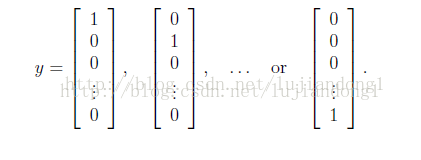
Y=zeros(m,num_labels);
for i=1:num_labels
Y(:,i)=(y==i);
end
-----------------------------------------------------------------------------------------------------------------------------------------------------------------
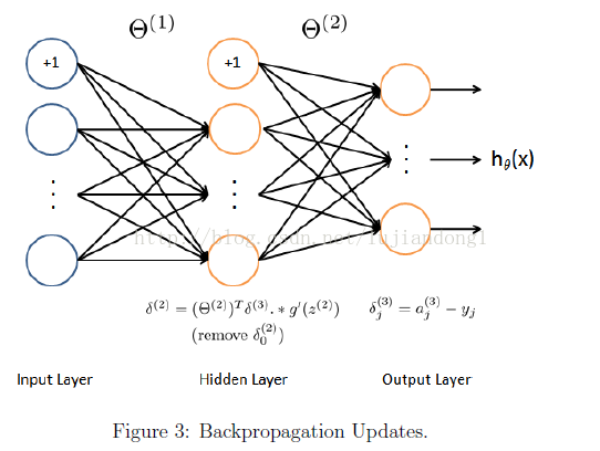
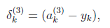
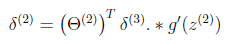
计算每一层的
delta3=zeros(m, num_labels);
for k = 1 : num_labels
delta3(:,k) = a3(:,k) - (y==k); %5000*10
end
delta2 = delta3 * Theta2 .* [ones(size(z2,1),1) sigmoidGradient(z2)]; %5000*26
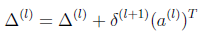
%compute Delta
Delta1 = delta2(:,2:end)' * a1; %25*401
Delta2 = delta3' * a2; %10*26
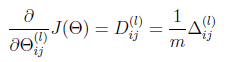
% compute Theta_grad
Theta1_grad = 1/m*Delta1;
Theta2_grad = 1/m*Delta2;
-------------------------------------------------------------------------------------------------------------------------------------------------
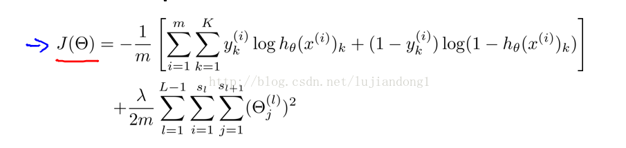
Regularized Neural Networks
% 正则化grad
reg1 = lambda/m*Theta1;
reg2 = lambda/m*Theta2;
reg1(:,1) = 0;
reg2(:,1) = 0;
Theta1_grad = Theta1_grad + reg1;
Theta2_grad = Theta2_grad + reg2;
---------------------------------------------------------------------------------------------------------------------------------------------------------------------------------------
Random initialization

% Randomly initialize the weights to small values
epsilon init = 0.12;
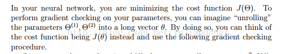
W = rand(L out, 1 + L in) * 2 * epsilon init − epsilon init;Gradient checking
梯度校验法是本周课程中非常值得学习的技巧。首先一个问题,如何判断我们神经网络中计算梯度(代价函数的导数是否是正确的呢)。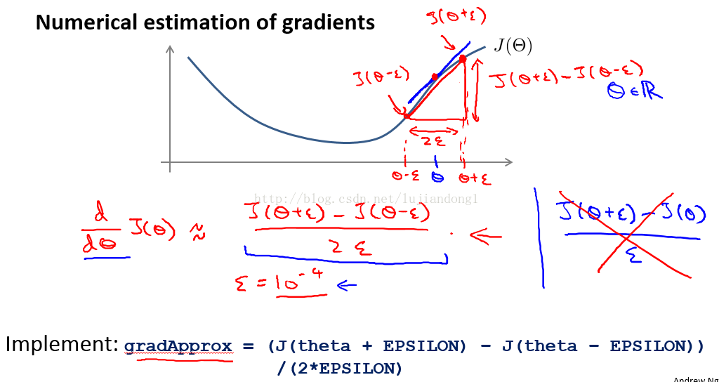
function checkNNGradients(lambda)
%CHECKNNGRADIENTS Creates a small neural network to check the
%backpropagation gradients
%   CHECKNNGRADIENTS(lambda) Creates a small neural network to check the
%   backpropagation gradients, it will output the analytical gradients
%   produced by your backprop code and the numerical gradients (computed
%   using computeNumericalGradient). These two gradient computations should
%   result in very similar values.
%

if ~exist('lambda', 'var') || isempty(lambda)
    lambda = 0;
end

input_layer_size = 3;
hidden_layer_size = 5;
num_labels = 3;
m = 5;

% We generate some 'random' test data
Theta1 = debugInitializeWeights(hidden_layer_size, input_layer_size);
Theta2 = debugInitializeWeights(num_labels, hidden_layer_size);
% Reusing debugInitializeWeights to generate X
X  = debugInitializeWeights(m, input_layer_size - 1);
y  = 1 + mod(1:m, num_labels)';

% Unroll parameters
nn_params = [Theta1(:) ; Theta2(:)];

% Short hand for cost function
costFunc = @(p) nnCostFunction(p, input_layer_size, hidden_layer_size, ...
                               num_labels, X, y, lambda);

[cost, grad] = costFunc(nn_params);
numgrad = computeNumericalGradient(costFunc, nn_params);

% Visually examine the two gradient computations.  The two columns
% you get should be very similar.
disp([numgrad grad]);
fprintf(['The above two columns you get should be very similar.\n' ...
         '(Left-Your Numerical Gradient, Right-Analytical Gradient)\n\n']);

% Evaluate the norm of the difference between two solutions.
% If you have a correct implementation, and assuming you used EPSILON = 0.0001
% in computeNumericalGradient.m, then diff below should be less than 1e-9
diff = norm(numgrad-grad)/norm(numgrad+grad);

fprintf(['If your backpropagation implementation is correct, then \n' ...
         'the relative difference will be small (less than 1e-9). \n' ...
         '\nRelative Difference: %g\n'], diff);

end<span style="color:#ff0000;">
</span>num_labels, X, y, lambda);
%利用nnCostFunction计算相应参数下的梯度值
[cost, grad] = costFunc(nn_params);
numgrad = computeNumericalGradient(costFunc, nn_params);
% Visually examine the two gradient computations. The two columns
% you get should be very similar.
disp([numgrad grad]);
从函数的调用可知 numgrad = computeNumericalGradient(costFunc, nn_params);J就是nnCostFunction的函数指针
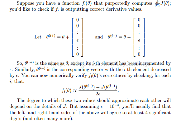
function numgrad = computeNumericalGradient(J, theta)
%COMPUTENUMERICALGRADIENT Computes the gradient using "finite differences"
%and gives us a numerical estimate of the gradient.
%   numgrad = COMPUTENUMERICALGRADIENT(J, theta) computes the numerical
%   gradient of the function J around theta. Calling y = J(theta) should
%   return the function value at theta.

% Notes: The following code implements numerical gradient checking, and
%        returns the numerical gradient.It sets numgrad(i) to (a numerical
%        approximation of) the partial derivative of J with respect to the
%        i-th input argument, evaluated at theta. (i.e., numgrad(i) should
%        be the (approximately) the partial derivative of J with respect
%        to theta(i).)
%

numgrad = zeros(size(theta));
perturb = zeros(size(theta));
e = 1e-4;
for p = 1:numel(theta)
    % Set perturbation vector
    perturb(p) = e;
    loss1 = J(theta - perturb);
    loss2 = J(theta + perturb);
    % Compute Numerical Gradient
    numgrad(p) = (loss2 - loss1) / (2*e);
    perturb(p) = 0;
end

end
for p = 1:numel(theta)
% Set perturbation vector
perturb(p) = e;
%J就是nnCostFunction的函数指针,计算θ=theta - perturb,下的代价函数
loss1 = J(theta - perturb);
%计算θ=theta+perturb,下的代价函数
loss2 = J(theta + perturb);
% Compute Numerical Gradient
%数值计算公式求梯度。
numgrad(p) = (loss2 - loss1) / (2*e);
perturb(p) = 0;
end
Backpropagation
Sigmoid gradient
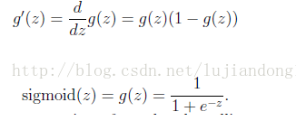
function g = sigmoidGradient(z)
%SIGMOIDGRADIENT returns the gradient of the sigmoid function
%evaluated at z
%   g = SIGMOIDGRADIENT(z) computes the gradient of the sigmoid function
%   evaluated at z. This should work regardless if z is a matrix or a
%   vector. In particular, if z is a vector or matrix, you should return
%   the gradient for each element.

g = zeros(size(z));

% ====================== YOUR CODE HERE ======================
% Instructions: Compute the gradient of the sigmoid function evaluated at
%               each value of z (z can be a matrix, vector or scalar).

g = sigmoid(z).*(1-sigmoid(z));

% =============================================================
end


 3193
3193


 被折叠的 条评论
为什么被折叠?
被折叠的 条评论
为什么被折叠?
 到【灌水乐园】发言


