Python: Neural Networks

这是用Python实现的Neural Networks, 基于Python 2.7.9, numpy, matplotlib。
代码来源于斯坦福大学的课程: http://cs231n.github.io/neural-networks-case-study/
基本是照搬过来,通过这个程序有助于了解python语法,以及Neural Networks 的原理。

import numpy as np
import matplotlib.pyplot as plt

N = 200 # number of points per class
D = 2 # dimensionality
K = 3 # number of classes
X = np.zeros((N*K,D)) # data matrix (each row = single example)
y = np.zeros(N*K, dtype='uint8') # class labels

for j in xrange(K):
  ix = range(N*j,N*(j+1))
  r = np.linspace(0.0,1,N) # radius
  t = np.linspace(j*4,(j+1)*4,N) + np.random.randn(N)*0.2 # theta
  X[ix] = np.c_[r*np.sin(t), r*np.cos(t)]
  y[ix] = j

# print y

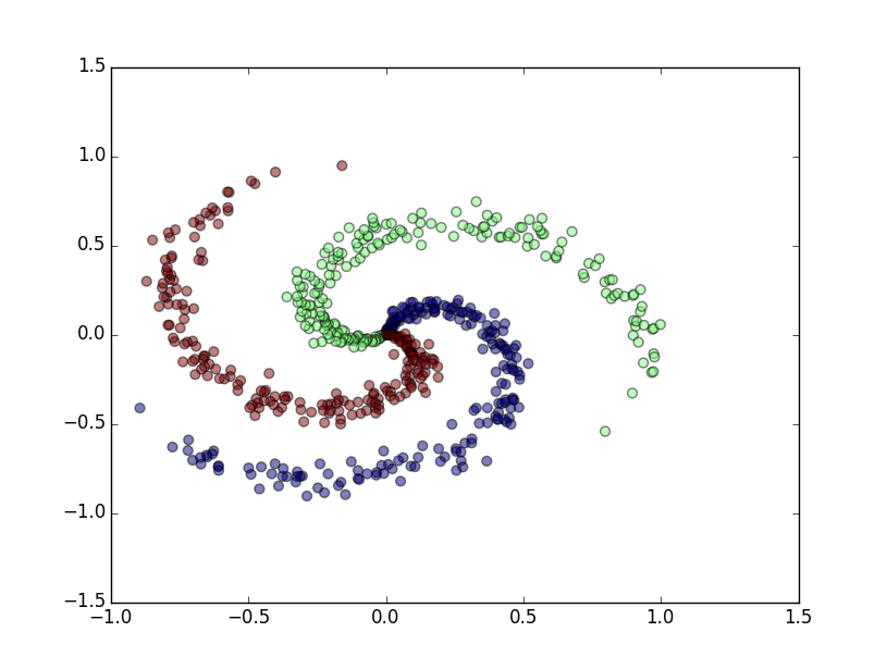
# lets visualize the data:
plt.scatter(X[:,0], X[:,1], s=40, c=y, alpha=0.5)
plt.show()

# Train a Linear Classifier

# initialize parameters randomly

h = 20 # size of hidden layer
W = 0.01 * np.random.randn(D,h)
b = np.zeros((1,h))
W2 = 0.01 * np.random.randn(h,K)
b2 = np.zeros((1,K))

# define some hyperparameters
step_size = 1e-0
reg = 1e-3 # regularization strength

# gradient descent loop
num_examples = X.shape[0]
for i in xrange(1):

  # evaluate class scores, [N x K]
  hidden_layer = np.maximum(0, np.dot(X, W) + b) # note, ReLU activation
  # print np.size(hidden_layer,1)
  scores = np.dot(hidden_layer, W2) + b2

  # compute the class probabilities
  exp_scores = np.exp(scores)
  probs = exp_scores / np.sum(exp_scores, axis=1, keepdims=True) # [N x K]

  # compute the loss: average cross-entropy loss and regularization
  corect_logprobs = -np.log(probs[range(num_examples),y])
  data_loss = np.sum(corect_logprobs)/num_examples
  reg_loss = 0.5*reg*np.sum(W*W) + 0.5*reg*np.sum(W2*W2)
  loss = data_loss + reg_loss
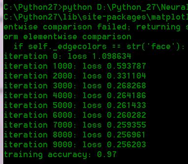
  if i % 1000 == 0:
    print "iteration %d: loss %f" % (i, loss)

  # compute the gradient on scores
  dscores = probs
  dscores[range(num_examples),y] -= 1
  dscores /= num_examples

  # backpropate the gradient to the parameters
  # first backprop into parameters W2 and b2
  dW2 = np.dot(hidden_layer.T, dscores)
  db2 = np.sum(dscores, axis=0, keepdims=True)
  # next backprop into hidden layer
  dhidden = np.dot(dscores, W2.T)
  # backprop the ReLU non-linearity
  dhidden[hidden_layer <= 0] = 0

  # finally into W,b
  dW = np.dot(X.T, dhidden)
  db = np.sum(dhidden, axis=0, keepdims=True)

  # add regularization gradient contribution
  dW2 += reg * W2
  dW += reg * W

  # perform a parameter update
  W += -step_size * dW
  b += -step_size * db
  W2 += -step_size * dW2
  b2 += -step_size * db2

  # evaluate training set accuracy
hidden_layer = np.maximum(0, np.dot(X, W) + b)
scores = np.dot(hidden_layer, W2) + b2
predicted_class = np.argmax(scores, axis=1)

print 'training accuracy: %.2f' % (np.mean(predicted_class == y))

随机生成的数据

这里写图片描述

运行结果

这里写图片描述

eep Learning: Recurrent Neural Networks in Python: LSTM, GRU, and more RNN machine learning architectures in Python and Theano (Machine Learning in Python) by LazyProgrammer English | 8 Aug 2016 | ASIN: B01K31SQQA | 86 Pages | AZW3/MOBI/EPUB/PDF (conv) | 1.44 MB Like Markov models, Recurrent Neural Networks are all about learning sequences - but whereas Markov Models are limited by the Markov assumption, Recurrent Neural Networks are not - and as a result, they are more expressive, and more powerful than anything we’ve seen on tasks that we haven’t made progress on in decades. In the first section of the course we are going to add the concept of time to our neural networks. I’ll introduce you to the Simple Recurrent Unit, also known as the Elman unit. We are going to revisit the XOR problem, but we’re going to extend it so that it becomes the parity problem - you’ll see that regular feedforward neural networks will have trouble solving this problem but recurrent networks will work because the key is to treat the input as a sequence. In the next section of the book, we are going to revisit one of the most popular applications of recurrent neural networks - language modeling. One popular application of neural networks for language is word vectors or word embeddings. The most common technique for this is called Word2Vec, but I’ll show you how recurrent neural networks can also be used for creating word vectors. In the section after, we’ll look at the very popular LSTM, or long short-term memory unit, and the more modern and efficient GRU, or gated recurrent unit, which has been proven to yield comparable performance. We’ll apply these to some more practical problems, such as learning a language model from Wikipedia data and visualizing the word embeddings we get as a result. All of the materials required for this course can be downloaded and installed for FREE. We will do most of our work in Numpy, Matplotlib, and Theano. I am always available to answer
下面是使用Python实现NEURAL NETWORKS Uplift model for multiple correlated responses WITH LOWRANK REGULARIZATION的代码示例: ```python import numpy as np import pandas as pd import tensorflow as tf from sklearn.model_selection import train_test_split # 导入数据集 data = pd.read_csv('data.csv') X = data.drop(['response', 'treatment'], axis=1).values y = data['response'].values t = data['treatment'].values # 将数据集分为训练集和测试集 X_train, X_test, y_train, y_test, t_train, t_test = train_test_split(X, y, t, test_size=0.2) # 定义常量 n_features = X.shape[1] n_components = 5 alpha = 0.01 # 定义占位符 X_ph = tf.placeholder(tf.float32, shape=[None, n_features], name='X') y_ph = tf.placeholder(tf.float32, shape=[None], name='y') t_ph = tf.placeholder(tf.float32, shape=[None], name='t') # 定义神经网络模型 hidden_layer_1 = tf.layers.dense(X_ph, 64, activation=tf.nn.relu) hidden_layer_2 = tf.layers.dense(hidden_layer_1, 32, activation=tf.nn.relu) y_pred = tf.layers.dense(hidden_layer_2, 1, activation=tf.nn.sigmoid) # 定义损失函数 treated = tf.cast(tf.equal(t_ph, 1), tf.float32) control = 1 - treated uplift = tf.reduce_mean((y_pred * treated - y_pred * control)) mse = tf.reduce_mean(tf.square(y_pred - y_ph)) lowrank = tf.reduce_sum(tf.svd(tf.transpose(hidden_layer_1), compute_uv=False)) loss = mse - alpha * uplift + alpha * lowrank # 定义优化器 optimizer = tf.train.AdamOptimizer(learning_rate=0.001) train_step = optimizer.minimize(loss) # 定义会话 sess = tf.Session() sess.run(tf.global_variables_initializer()) # 训练模型 for i in range(100): _, loss_value, uplift_value, mse_value, lowrank_value = sess.run([train_step, loss, uplift, mse, lowrank], feed_dict={X_ph: X_train, y_ph: y_train, t_ph: t_train}) print('Epoch %d - Loss: %.4f, Uplift: %.4f, MSE: %.4f, Lowrank: %.4f' % (i, loss_value, uplift_value, mse_value, lowrank_value)) # 预测响应变量的值 y_train_pred = sess.run(y_pred, feed_dict={X_ph: X_train}) y_test_pred = sess.run(y_pred, feed_dict={X_ph: X_test}) # 计算控制组和干预组之间的差异 uplift_train = np.mean(y_train_pred[t_train == 1] - y_train_pred[t_train == 0]) uplift_test = np.mean(y_test_pred[t_test == 1] - y_test_pred[t_test == 0]) # 输出结果 print('Train uplift: %.2f' % uplift_train) print('Test uplift: %.2f' % uplift_test) ``` 请注意,这只是一个简单的示例,实际实现可能涉及更多的数据预处理和模型调整。
评论 2
添加红包

请填写红包祝福语或标题

红包个数最小为10个

红包金额最低5元

当前余额3.43前往充值 >
需支付:10.00
成就一亿技术人!
领取后你会自动成为博主和红包主的粉丝 规则
hope_wisdom
发出的红包
实付
使用余额支付
点击重新获取
扫码支付
钱包余额 0

抵扣说明:

1.余额是钱包充值的虚拟货币,按照1:1的比例进行支付金额的抵扣。
2.余额无法直接购买下载,可以购买VIP、付费专栏及课程。

余额充值