《Machine Learning（Tom M. Mitchell）》读书笔记——5、第四章

1. Introduction (about machine learning)

2. Concept Learning and the General-to-Specific Ordering

3. Decision Tree Learning

4. Artificial Neural Networks

5. Evaluating Hypotheses

6. Bayesian Learning

7. Computational Learning Theory

8. Instance-Based Learning

9. Genetic Algorithms

10. Learning Sets of Rules

11. Analytical Learning

12. Combining Inductive and Analytical Learning

13. Reinforcement Learning

4. Artificial Neural Networks

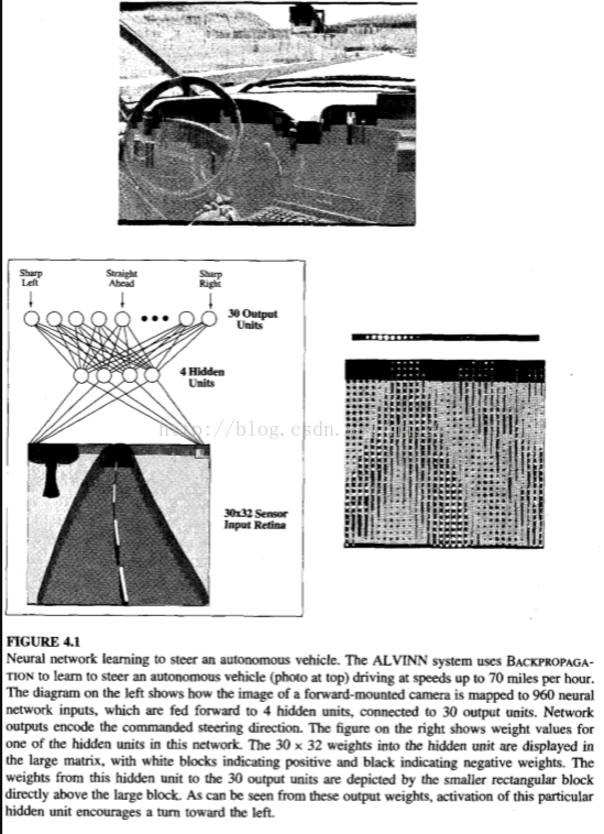
Artificial neural networks (ANNs) provide a general, practical method for learning real-valued, discrete-valued, and vector-valued functions from examples. Algorithms such as BACKPROPAGATION use gradient descent to tune network parameters to best fit a training set of input-output pairs. ANN learning is robust to errors in the training data and has been successfully applied to problems such as interpreting visual scenes, speech recognition, and learning robot control strategies.

4.2 NEURAL NETWORK REPRESENTATIONS

These are called "hidden" units because their output is available only within the network and is not available as part of the global network output. 

The network structure of ALYINN is typical of many ANNs. Here the individual units are interconnected in layers that form a directed acyclic graph(DAG, 有向无环图). In general, ANNs can be graphs with many types of structures-acyclic or cyclic, directed or undirected. This chapter will focus on the most common and practical ANN approaches, which are based on the BACKPROPAGATION algorithm(反向传播). The BACK- PROPAGATION algorithm assumes the network is a fixed structure that corresponds to a directed graph, possibly containing cycles. Learning corresponds to choosing a weight value for each edge in the graph. Although certain types of cycles are allowed, the vast majority of practical applications involve acyclic feed-forward networks, similar to the network structure used by ALVINN. 

4.3 APPROPRIATE PROBLEMS FOR NEURAL NETWORK LEARNING

 It is appropriate for problems with the following characteristics:

Instances are represented by many attribute-value pairs. 

The target function output may be discrete-valued, real-valued, or a vector of several real- or discrete-valued attributes.

The training examples may contain errors.

Long training times are acceptable.

Fast evaluation of the learned target function may be required. Although ANN learning times are relatively long, evaluating the learned network, in order to apply it to a subsequent instance, is typically very fast. For example, ALVINN applies its neural network several times per second to continually update its steering command as the vehicle drives forward. 

The ability of humans to understand the learned target function is not important.

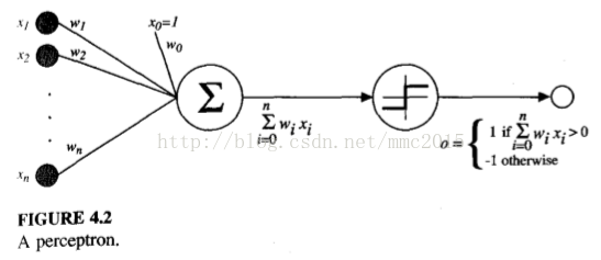
4.4 PERCEPTRON - the most simple ANN system

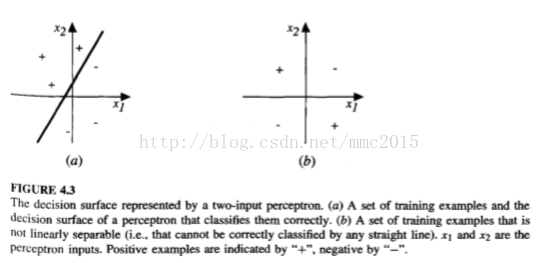
4.4.1 Representational Power of Perceptron

In fact, AND and OR can be viewed as special cases of m-of-n functions: that is, functions where at least m of the n inputs to the perceptron must be true. The OR function corresponds to rn = 1 and the AND function to m = n. Any m-of-n function is easily represented using a perceptron by setting all input weights to the same value (e.g., 0.5) and then setting the threshold wo accordingly.

In fact, every boolean function can be represented by some network of perceptrons only two levels deep, in which the inputs are fed to multiple units, and the outputs of these units are then input to a second, final stage. 

4.4.2 The Perceptron Training Rule

Let us begin by understanding how to learn the weights for a single perceptron. Here the precise learning problem is to determine a weight vector that causes the perceptron to produce the correct f 1 output for each of the given training examples. Several algorithms are known to solve this learning problem. Here we consider two: the perceptron rule and the delta rule (a variant of the LMS rule used in Chapter 1 for learning evaluation functions).

One way to learn an acceptable weight vector is to begin with random weights, then iteratively apply the perceptron to each training example, modifying the perceptron weights whenever it misclassifies an example. This process is repeated, iterating through the training examples as many times