CHAPTER 3 Improving the way neural networks learn

When a golf player is first learning to play golf, they usually spendmost of their time developing a basic swing. Only gradually do theydevelop other shots, learning to chip, draw and fade the ball,building on and modifying their basic swing. In a similar way, up tonow we've focused on understanding the backpropagation algorithm.It's our "basic swing", the foundation for learning in most work onneural networks. In this chapter I explain a suite of techniqueswhich can be used to improve on our vanilla implementation ofbackpropagation, and so improve the way our networks learn.

The techniques we'll develop in this chapter include: a better choiceof cost function, known asthe cross-entropy cost function; four so-called"regularization" methods (L1 and L2 regularization, dropout, and artificialexpansion of the training data), which make our networks better atgeneralizing beyond the training data; abetter method for initializing the weights in the network; and aset of heuristics to help choose good hyper-parameters for the network.I'll also overview several other techniques in less depth. The discussions are largely independentof one another, and so you may jump ahead if you wish. We'll alsoimplementmany of the techniques in running code, and use them to improve theresults obtained on the handwriting classification problem studied inChapter 1.

Of course, we're only covering a few of the many, many techniqueswhich have been developed for use in neural nets. The philosophy isthat the best entree to the plethora of available techniques isin-depth study of a few of the most important. Mastering thoseimportant techniques is not just useful in its own right, but willalso deepen your understanding of what problems can arise when you useneural networks. That will leave you well prepared to quickly pick upother techniques, as you need them.

The cross-entropy cost function

Most of us find it unpleasant to be wrong. Soon after beginning tolearn the piano I gave my first performance before an audience. I wasnervous, and began playing the piece an octave too low. I gotconfused, and couldn't continue until someone pointed out my error. Iwas very embarrassed. Yet while unpleasant, we also learn quickly whenwe're decisively wrong. You can bet that the next time I playedbefore an audience I played in the correct octave! By contrast, welearn more slowly when our errors are less well-defined.

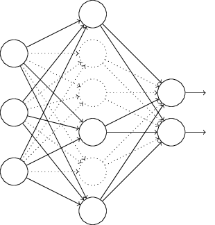
Ideally, we hope and expect that our neural networks will learn fastfrom their errors. Is this what happens in practice? To answer thisquestion, let's look at a toy example. The example involves a neuronwith just one input:

We'll train this neuron to do something ridiculously easy: take theinput 1

to the output 0

. Of course, this is such a trivial taskthat we could easily figure out an appropriate weight and bias byhand, without using a learning algorithm. However, it turns out to beilluminating to use gradient descent to attempt to learn a weight andbias. So let's take a look at how the neuron learns.

To make things definite, I'll pick the initial weight to be 0.6

andthe initial bias to be 0.9 . These are generic choices used as aplace to begin learning, I wasn't picking them to be special in anyway. The initial output from the neuron is 0.82 , so quite a bit oflearning will be needed before our neuron gets near the desiredoutput, 0.0 . Click on "Run" in the bottom right corner below tosee how the neuron learns an output much closer to 0.0 . Note thatthis isn't a pre-recorded animation, your browser is actuallycomputing the gradient, then using the gradient to update the weightand bias, and displaying the result. The learning rate is η=0.15 , which turns out to be slow enough that we can follow what'shappening, but fast enough that we can get substantial learning injust a few seconds. The cost is the quadratic cost function, C

,introduced back in Chapter 1. I'll remind you of the exact form ofthe cost function shortly, so there's no need to go and dig up thedefinition. Note that you can run the animation multiple times byclicking on "Run" again.

As you can see, the neuron rapidly learns a weight and bias thatdrives down the cost, and gives an output from the neuron of about 0.09

. That's not quite the desired output, 0.0 , but it is prettygood. Suppose, however, that we instead choose both the startingweight and the starting bias to be 2.0 . In this case the initialoutput is 0.98 , which is very badly wrong. Let's look at how theneuron learns to output 0

in this case. Click on "Run" again:

Although this example uses the same learning rate ( η=0.15

), wecan see that learning starts out much more slowly. Indeed, for thefirst 150 or so learning epochs, the weights and biases don't changemuch at all. Then the learning kicks in and, much as in our firstexample, the neuron's output rapidly moves closer to 0.0

.

This behaviour is strange when contrasted to human learning. As Isaid at the beginning of this section, we often learn fastest whenwe're badly wrong about something. But we've just seen that ourartificial neuron has a lot of difficulty learning when it's badlywrong - far more difficulty than when it's just a little wrong.What's more, it turns out that this behaviour occurs not just in thistoy model, but in more general networks. Why is learning so slow?And can we find a way of avoiding this slowdown?

To understand the origin of the problem, consider that our neuronlearns by changing the weight and bias at a rate determined by thepartial derivatives of the cost function, ∂C/∂w

and ∂C/∂b . So saying "learning is slow" is reallythe same as saying that those partial derivatives are small. Thechallenge is to understand why they are small. To understand that,let's compute the partial derivatives. Recall that we're using thequadratic cost function, which, fromEquation (6), is given by

C=(y−a)22,(54)

where a is the neuron's output when the training input x=1 isused, and y=0 is the corresponding desired output. To write thismore explicitly in terms of the weight and bias, recall that a=σ(z) , where z=wx+b . Using the chain rule to differentiatewith respect to the weight and bias we get

∂C∂w∂C∂b==(a−y)σ′(z)x=aσ′(z)(a−y)σ′(z)=aσ′(z),(55)(56)

where I have substituted x=1 and y=0 . To understand thebehaviour of these expressions, let's look more closely at the σ′(z) term on the right-hand side. Recall the shape of the σ

function:

-4-3-2-1012340.00.20.40.60.81.0zsigmoid function

We can see from this graph that when the neuron's output is close to 1

, the curve gets very flat, and so σ′(z) gets very small.Equations (55) and (56) then tell us that ∂C/∂w and ∂C/∂b

get verysmall. This is the origin of the learning slowdown. What's more, aswe shall see a little later, the learning slowdown occurs foressentially the same reason in more general neural networks, not justthe toy example we've been playing with.

Introducing the cross-entropy cost function

How can we address the learning slowdown? It turns out that we cansolve the problem by replacing the quadratic cost with a differentcost function, known as the cross-entropy. To understand thecross-entropy, let's move a little away from our super-simple toymodel. We'll suppose instead that we're trying to train a neuron withseveral input variables, x1,x2,…

, corresponding weights w1,w2,… , and a bias, b

:

The output from the neuron is, of course, a=σ(z) , where z=∑jwjxj+b is the weighted sum of the inputs. We define thecross-entropy cost function for this neuron by

C=−1n∑x[ylna+(1−y)ln(1−a)],(57)

where n is the total number of items of training data, the sum isover all training inputs, x , and y is the corresponding desiredoutput.

It's not obvious that the expression (57)fixes the learning slowdown problem. In fact, frankly, it's not evenobvious that it makes sense to call this a cost function! Beforeaddressing the learning slowdown, let's see in what sense thecross-entropy can be interpreted as a cost function.

Two properties in particular make it reasonable to interpret thecross-entropy as a cost function. First, it's non-negative, that is, C>0

. To see this, notice that: (a) all the individual terms inthe sum in (57) are negative, since bothlogarithms are of numbers in the range 0 to 1

; and (b) there is aminus sign out the front of the sum.

Second, if the neuron's actual output is close to the desired outputfor all training inputs, x

, then the cross-entropy will be close tozero* *To prove this I will need to assume that the desired outputs y are all either 0 or 1 . This is usually the case when solving classification problems, for example, or when computing Boolean functions. To understand what happens when we don't make this assumption, see the exercises at the end of this section.. Tosee this, suppose for example that y=0 and a≈0 for someinput x . This is a case when the neuron is doing a good job on thatinput. We see that the first term in theexpression (57) for the cost vanishes, since y=0 , while the second term is just −ln(1−a)≈0 . Asimilar analysis holds when y=1 and a≈1

. And so thecontribution to the cost will be low provided the actual output isclose to the desired output.

Summing up, the cross-entropy is positive, and tends toward zero asthe neuron gets better at computing the desired output, y

, for alltraining inputs, x . These are both properties we'd intuitivelyexpect for a cost function. Indeed, both properties are alsosatisfied by the quadratic cost. So that's good news for thecross-entropy. But the cross-entropy cost function has the benefitthat, unlike the quadratic cost, it avoids the problem of learningslowing down. To see this, let's compute the partial derivative ofthe cross-entropy cost with respect to the weights. We substitute a=σ(z) into (57), and apply the chainrule twice, obtaining:

∂C∂wj==−1n∑x(yσ(z)−(1−y)1−σ(z))∂σ∂wj−1n∑x(yσ(z)−(1−y)1−σ(z))σ′(z)xj.(58)(59)

Putting everything over a common denominator and simplifying thisbecomes:

∂C∂wj=1n∑xσ′(z)xjσ(z)(1−σ(z))(σ(z)−y).(60)

Using the definition of the sigmoid function, σ(z)=1/(1+e−z) , and a little algebra we can show that σ′(z)=σ(z)(1−σ(z)) . I'll ask you to verify this in an exercisebelow, but for now let's accept it as given. We see that the σ′(z) and σ(z)(1−σ(z)) terms cancel in the equationjust above, and it simplifies to become:

∂C∂wj=1n∑xxj(σ(z)−y).(61)

This is a beautiful expression. It tells us that the rate at whichthe weight learns is controlled by σ(z)−y , i.e., by the errorin the output. The larger the error, the faster the neuron willlearn. This is just what we'd intuitively expect. In particular, itavoids the learning slowdown caused by the σ′(z) term in theanalogous equation for the quadratic cost, Equation (55).When we use the cross-entropy, the σ′(z)

term gets canceledout, and we no longer need worry about it being small. Thiscancellation is the special miracle ensured by the cross-entropy costfunction. Actually, it's not really a miracle. As we'll see later,the cross-entropy was specially chosen to have just this property.

In a similar way, we can compute the partial derivative for the bias.I won't go through all the details again, but you can easily verifythat

∂C∂b=1n∑x(σ(z)−y).(62)

Again, this avoids the learning slowdown caused by the σ′(z)

term in the analogous equation for the quadratic cost,Equation (56).

Exercise

• Verify that σ′(z)=σ(z)(1−σ(z))

• .

Let's return to the toy example we played with earlier, and explorewhat happens when we use the cross-entropy instead of the quadraticcost. To re-orient ourselves, we'll begin with the case where thequadratic cost did just fine, with starting weight 0.6

and startingbias 0.9

. Press "Run" to see what happens when we replace thequadratic cost by the cross-entropy:

Unsurprisingly, the neuron learns perfectly well in this instance,just as it did earlier. And now let's look at the case where ourneuron got stuck before (link, forcomparison), with the weight and bias both starting at 2.0

:

Success! This time the neuron learned quickly, just as we hoped. Ifyou observe closely you can see that the slope of the cost curve wasmuch steeper initially than the initial flat region on thecorresponding curve for the quadratic cost. It's that steepness whichthe cross-entropy buys us, preventing us from getting stuck just whenwe'd expect our neuron to learn fastest, i.e., when the neuron startsout badly wrong.

I didn't say what learning rate was used in the examples justillustrated. Earlier, with the quadratic cost, we used η=0.15

.Should we have used the same learning rate in the new examples? Infact, with the change in cost function it's not possible to sayprecisely what it means to use the "same" learning rate; it's anapples and oranges comparison. For both cost functions I simplyexperimented to find a learning rate that made it possible to see whatis going on. If you're still curious, despite my disavowal, here'sthe lowdown: I used η=0.005

in the examples just given.

You might object that the change in learning rate makes the graphsabove meaningless. Who cares how fast the neuron learns, when ourchoice of learning rate was arbitrary to begin with?! That objectionmisses the point. The point of the graphs isn't about the absolutespeed of learning. It's about how the speed of learning changes. Inparticular, when we use the quadratic cost learning is slowerwhen the neuron is unambiguously wrong than it is later on, as theneuron gets closer to the correct output; while with the cross-entropylearning is faster when the neuron is unambiguously wrong. Thosestatements don't depend on how the learning rate is set.

We've been studying the cross-entropy for a single neuron. However,it's easy to generalize the cross-entropy to many-neuron multi-layernetworks. In particular, suppose y=y1,y2,…

are thedesired values at the output neurons, i.e., the neurons in the finallayer, while aL1,aL2,… are the actual output values.Then we define the cross-entropy by

C=−1n∑x∑j[yjlnaLj+(1−yj)ln(1−aLj)].(63)

This is the same as our earlier expression,Equation (57), except now we've got the ∑j

summing over all the output neurons. I won't explicitly workthrough a derivation, but it should be plausible that using theexpression (63) avoids a learning slowdown inmany-neuron networks. If you're interested, you can work through thederivation in the problem below.

When should we use the cross-entropy instead of the quadratic cost?In fact, the cross-entropy is nearly always the better choice,provided the output neurons are sigmoid neurons. To see why, considerthat when we're setting up the network we usually initialize theweights and biases using some sort of randomization. It may happenthat those initial choices result in the network being decisivelywrong for some training input - that is, an output neuron will havesaturated near 1

, when it should be 0

, or vice versa. If we'reusing the quadratic cost that will slow down learning. It won't stoplearning completely, since the weights will continue learning fromother training inputs, but it's obviously undesirable.

Exercises

• One gotcha with the cross-entropy is that it can be difficult at first to remember the respective roles of the y

s and the a s. It's easy to get confused about whether the right form is −[ylna+(1−y)ln(1−a)] or −[alny+(1−a)ln(1−y)] . What happens to the second of these expressions when y=0 or 1

• ? Does this problem afflict the first expression? Why or why not?
• In the single-neuron discussion at the start of this section, I argued that the cross-entropy is small if σ(z)≈y for all training inputs. The argument relied on y being equal to either 0 or 1 . This is usually true in classification problems, but for other problems (e.g., regression problems) y can sometimes take values intermediate between 0 and 1 . Show that the cross-entropy is still minimized when σ(z)=y for all training inputs. When this is the case the cross-entropy has the value:
  C=−1n∑x[ylny+(1−y)ln(1−y)].(64)
  The quantity −[ylny+(1−y)ln(1−y)]
  • is sometimes known as the binary entropy.

  Problems

  • Many-layer multi-neuron networks In the notation introduced in the last chapter, show that for the quadratic cost the partial derivative with respect to weights in the output layer is
    ∂C∂wLjk=1n∑xaL−1k(aLj−yj)σ′(zLj).(65)
  The term σ′(zLj) causes a learning slowdown whenever an output neuron saturates on the wrong value. Show that for the cross-entropy cost the output error δL for a single training example x is given by
  δL=aL−y.(66)
  Use this expression to show that the partial derivative with respect to the weights in the output layer is given by
  ∂C∂wLjk=1n∑xaL−1k(aLj−yj).(67)
  The σ′(zLj)
• term has vanished, and so the cross-entropy avoids the problem of learning slowdown, not just when used with a single neuron, as we saw earlier, but also in many-layer multi-neuron networks. A simple variation on this analysis holds also for the biases. If this is not obvious to you, then you should work through that analysis as well.
• Using the quadratic cost when we have linear neurons in the output layer Suppose that we have a many-layer multi-neuron network. Suppose all the neurons in the final layer are linear neurons, meaning that the sigmoid activation function is not applied, and the outputs are simply aLj=zLj . Show that if we use the quadratic cost function then the output error δL for a single training example x is given by
  δL=aL−y.(68)
  Similarly to the previous problem, use this expression to show that the partial derivatives with respect to the weights and biases in the output layer are given by
  ∂C∂wLjk∂C∂bLj==1n∑xaL−1k(aLj−yj)1n∑x(aLj−yj).(69)(70)
  • This shows that if the output neurons are linear neurons then the quadratic cost will not give rise to any problems with a learning slowdown. In this case the quadratic cost is, in fact, an appropriate cost function to use.

  Using the cross-entropy to classify MNIST digits

  The cross-entropy is easy to implement as part of a program whichlearns using gradient descent and backpropagation. We'll do thatlater in the chapter, developing an improved version of ourearlier program for classifying the MNIST handwritten digits,network.py. The new program is called network2.py, andincorporates not just the cross-entropy, but also several othertechniques developed in this chapter**The code is available on GitHub.. For now, let's look at how well our new programclassifies MNIST digits. As was the case in Chapter 1, we'll use anetwork with 30

  hidden neurons, and we'll use a mini-batch size of 10 . We set the learning rate to η=0.5 **In Chapter 1 we used the quadratic cost and a learning rate of η=3.0 . As discussed above, it's not possible to say precisely what it means to use the "same" learning rate when the cost function is changed. For both cost functions I experimented to find a learning rate that provides near-optimal performance, given the other hyper-parameter choices.
  
  There is, incidentally, a very rough general heuristic for relating the learning rate for the cross-entropy and the quadratic cost. As we saw earlier, the gradient terms for the quadratic cost have an extra σ′=σ(1−σ) term in them. Suppose we average this over values for σ , ∫10dσσ(1−σ)=1/6 . We see that (very roughly) the quadratic cost learns an average of 6 times slower, for the same learning rate. This suggests that a reasonable starting point is to divide the learning rate for the quadratic cost by 6 . Of course, this argument is far from rigorous, and shouldn't be taken too seriously. Still, it can sometimes be a useful starting point. and we train for 30

  epochs.The interface to network2.py is slightly different thannetwork.py, but it should still be clear what is going on. Youcan, by the way, get documentation about network2.py'sinterface by using commands such as help(network2.Network.SGD)in a Python shell.

  >>> import mnist_loader
  >>> training_data, validation_data, test_data = \
  ... mnist_loader.load_data_wrapper()
  >>> import network2
  >>> net = network2.Network([784, 30, 10], cost=network2.CrossEntropyCost)
  >>> net.large_weight_initializer()
  >>> net.SGD(training_data, 30, 10, 0.5, evaluation_data=test_data,
  ... monitor_evaluation_accuracy=True)
  

  Note, by the way, that the net.large_weight_initializer()command is used to initialize the weights and biases in the same wayas described in Chapter 1. We need to run this command because laterin this chapter we'll change the default weight initialization in ournetworks. The result from running the above sequence of commands is anetwork with 95.49

  percent accuracy. This is pretty close to theresult we obtained in Chapter 1, 95.42

  percent, using the quadraticcost.

  Let's look also at the case where we use 100

  hidden neurons, thecross-entropy, and otherwise keep the parameters the same. In thiscase we obtain an accuracy of 96.82 percent. That's a substantialimprovement over the results from Chapter 1, where we obtained aclassification accuracy of 96.59 percent, using the quadratic cost.That may look like a small change, but consider that the error ratehas dropped from 3.41 percent to 3.18

  percent. That is, we'veeliminated about one in fourteen of the original errors. That's quitea handy improvement.

  It's encouraging that the cross-entropy cost gives us similar orbetter results than the quadratic cost. However, these results don'tconclusively prove that the cross-entropy is a better choice. Thereason is that I've put only a little effort into choosinghyper-parameters such as learning rate, mini-batch size, and so on.For the improvement to be really convincing we'd need to do a thoroughjob optimizing such hyper-parameters. Still, the results areencouraging, and reinforce our earlier theoretical argument that thecross-entropy is a better choice than the quadratic cost.

  This, by the way, is part of a general pattern that we'll see throughthis chapter and, indeed, through much of the rest of the book. We'lldevelop a new technique, we'll try it out, and we'll get "improved"results. It is, of course, nice that we see such improvements. Butthe interpretation of such improvements is always problematic.They're only truly convincing if we see an improvement after puttingtremendous effort into optimizing all the other hyper-parameters.That's a great deal of work, requiring lots of computing power, andwe're not usually going to do such an exhaustive investigation.Instead, we'll proceed on the basis of informal tests like those doneabove. Still, you should keep in mind that such tests fall short ofdefinitive proof, and remain alert to signs that the arguments arebreaking down.

  By now, we've discussed the cross-entropy at great length. Why go toso much effort when it gives only a small improvement to our MNISTresults? Later in the chapter we'll see other techniques - notably,regularization - whichgive much bigger improvements. So why so much focus on cross-entropy?Part of the reason is that the cross-entropy is a widely-used costfunction, and so is worth understanding well. But the more importantreason is that neuron saturation is an important problem in neuralnets, a problem we'll return to repeatedly throughout the book. Andso I've discussed the cross-entropy at length because it's a goodlaboratory to begin understanding neuron saturation and how it may beaddressed.

  What does the cross-entropy mean? Where does it come from?

  Our discussion of the cross-entropy has focused on algebraic analysisand practical implementation. That's useful, but it leaves unansweredbroader conceptual questions, like: what does the cross-entropy mean?Is there some intuitive way of thinking about the cross-entropy? Andhow could we have dreamed up the cross-entropy in the first place?

  Let's begin with the last of these questions: what could havemotivated us to think up the cross-entropy in the first place?Suppose we'd discovered the learning slowdown described earlier, andunderstood that the origin was the σ′(z)

  terms inEquations (55) and (56). After staring atthose equations for a bit, we might wonder if it's possible to choosea cost function so that the σ′(z) term disappeared. In thatcase, the cost C=Cx for a single training example x wouldsatisfy
  ∂C∂wj∂C∂b==xj(a−y)(a−y).(71)(72)
  If we could choose the cost function to make these equations true,then they would capture in a simple way the intuition that the greaterthe initial error, the faster the neuron learns. They'd alsoeliminate the problem of a learning slowdown. In fact, starting fromthese equations we'll now show that it's possible to derive the formof the cross-entropy, simply by following our mathematical noses. Tosee this, note that from the chain rule we have
  ∂C∂b=∂C∂aσ′(z).(73)
  Using σ′(z)=σ(z)(1−σ(z))=a(1−a) the last equationbecomes
  ∂C∂b=∂C∂aa(1−a).(74)
  Comparing to Equation (72) we obtain
  ∂C∂a=a−ya(1−a).(75)
  Integrating this expression with respect to a gives
  C=−[ylna+(1−y)ln(1−a)]+constant,(76)
  for some constant of integration. This is the contribution to thecost from a single training example, x . To get the full costfunction we must average over training examples, obtaining
  C=−1n∑x[ylna+(1−y)ln(1−a)]+constant,(77)

  where the constant here is the average of the individual constants foreach training example. And so we see thatEquations (71)and (72) uniquely determine the formof the cross-entropy, up to an overall constant term. Thecross-entropy isn't something that was miraculously pulled out of thinair. Rather, it's something that we could have discovered in a simpleand natural way.

  What about the intuitive meaning of the cross-entropy? How should wethink about it? Explaining this in depth would take us further afieldthan I want to go. However, it is worth mentioning that there is astandard way of interpreting the cross-entropy that comes from thefield of information theory. Roughly speaking, the idea is that thecross-entropy is a measure of surprise. In particular, our neuron istrying to compute the function x→y=y(x)

  . But insteadit computes the function x→a=a(x) . Suppose we thinkof a as our neuron's estimated probability that y is 1 , and 1−a is the estimated probability that the right value for y is 0 . Then the cross-entropy measures how "surprised" we are, onaverage, when we learn the true value for y

  . We get low surprise ifthe output is what we expect, and high surprise if the output isunexpected. Of course, I haven't said exactly what "surprise"means, and so this perhaps seems like empty verbiage. But in factthere is a precise information-theoretic way of saying what is meantby surprise. Unfortunately, I don't know of a good, short,self-contained discussion of this subject that's available online.But if you want to dig deeper, then Wikipedia contains abrief summary that will get you started down the right track. And thedetails can be filled in by working through the materials about theKraft inequality in chapter 5 of the book about information theory byCover and Thomas.

  Problem

  • We've discussed at length the learning slowdown that can occur when output neurons saturate, in networks using the quadratic cost to train. Another factor that may inhibit learning is the presence of the xj
  term in Equation (61). Because of this term, when an input xj is near to zero, the corresponding weight wj will learn slowly. Explain why it is not possible to eliminate the xj
  • term through a clever choice of cost function.

  Softmax

  In this chapter we'll mostly use the cross-entropy cost to address theproblem of learning slowdown. However, I want to briefly describeanother approach to the problem, based on what are calledsoftmax layers of neurons. We're not actually going to usesoftmax layers in the remainder of the chapter, so if you're in agreat hurry, you can skip to the next section. However, softmax isstill worth understanding, in part because it's intrinsicallyinteresting, and in part because we'll use softmax layers inChapter 6, in our discussion of deep neuralnetworks.

  The idea of softmax is to define a new type of output layer for ourneural networks. It begins in the same way as with a sigmoid layer,by forming the weighted inputs**In describing the softmax we'll make frequent use of notation introduced in the last chapter. You may wish to revisit that chapter if you need to refresh your memory about the meaning of the notation. zLj=∑kwLjkaL−1k+bLj

  . However,we don't apply the sigmoid function to get the output. Instead, in asoftmax layer we apply the so-called softmax function to the zLj . According to this function, the activation aLj of the j th output neuron is
  aLj=ezLj∑kezLk,(78)

  where in the denominator we sum over all the output neurons.

  If you're not familiar with the softmax function,Equation (78) may look pretty opaque. It's certainlynot obvious why we'd want to use this function. And it's also notobvious that this will help us address the learning slowdown problem.To better understand Equation (78), suppose we have anetwork with four output neurons, and four corresponding weightedinputs, which we'll denote zL1,zL2,zL3

  , and zL4 . Shownbelow are adjustable sliders showing possible values for the weightedinputs, and a graph of the corresponding output activations. A goodplace to start exploration is by using the bottom slider to increase zL4

  :

  zL1=

  aL1=

  zL2

  =

  aL2=

  zL3

  =

  aL3=

  zL4

  =

  aL4=

  As you increase zL4

  , you'll see an increase in the correspondingoutput activation, aL4 , and a decrease in the other outputactivations. Similarly, if you decrease zL4 then aL4 willdecrease, and all the other output activations will increase. Infact, if you look closely, you'll see that in both cases the totalchange in the other activations exactly compensates for the change in aL4 . The reason is that the output activations are guaranteed toalways sum up to 1 , as we can prove usingEquation (78) and a little algebra:
  ∑jaLj=∑jezLj∑kezLk=1.(79)
  As a result, if aL4 increases, then the other output activationsmust decrease by the same total amount, to ensure the sum over allactivations remains 1

  . And, of course, similar statements hold forall the other activations.

  Equation (78) also implies that the output activationsare all positive, since the exponential function is positive.Combining this with the observation in the last paragraph, we see thatthe output from the softmax layer is a set of positive numbers whichsum up to 1

  . In other words, the output from the softmax layer canbe thought of as a probability distribution.

  The fact that a softmax layer outputs a probability distribution israther pleasing. In many problems it's convenient to be able tointerpret the output activation aLj

  as the network's estimate ofthe probability that the correct output is j . So, for instance, inthe MNIST classification problem, we can interpret aLj as thenetwork's estimated probability that the correct digit classificationis j

  .

  By contrast, if the output layer was a sigmoid layer, then wecertainly couldn't assume that the activations formed a probabilitydistribution. I won't explicitly prove it, but it should be plausiblethat the activations from a sigmoid layer won't in general form aprobability distribution. And so with a sigmoid output layer we don'thave such a simple interpretation of the output activations.

  Exercise

  • Construct an example showing explicitly that in a network with a sigmoid output layer, the output activations aLj
  won't always sum to 1
  • .

  We're starting to build up some feel for the softmax function and theway softmax layers behave. Just to review where we're at: theexponentials in Equation (78) ensure that all the outputactivations are positive. And the sum in the denominator ofEquation (78) ensures that the softmax outputs sum to 1

  . So that particular form no longer appears so mysterious: rather,it is a natural way to ensure that the output activations form aprobability distribution. You can think of softmax as a way ofrescaling the zLj

  , and then squishing them together to form aprobability distribution.

  Exercises

  • Monotonicity of softmax Show that ∂aLj/∂zLk
  is positive if j=k and negative if j≠k . As a consequence, increasing zLj is guaranteed to increase the corresponding output activation, aLj
• , and will decrease all the other output activations. We already saw this empirically with the sliders, but this is a rigorous proof.
• Non-locality of softmax A nice thing about sigmoid layers is that the output aLj is a function of the corresponding weighted input, aLj=σ(zLj) . Explain why this is not the case for a softmax layer: any particular output activation aLj
  • depends on all the weighted inputs.

  Problem

  • Inverting the softmax layer Suppose we have a neural network with a softmax output layer, and the activations aLj
  are known. Show that the corresponding weighted inputs have the form zLj=lnaLj+C , for some constant C that is independent of j
  • .

  The learning slowdown problem: We've now built upconsiderable familiarity with softmax layers of neurons. But wehaven't yet seen how a softmax layer lets us address the learningslowdown problem. To understand that, let's define thelog-likelihood cost function. We'll use x

  to denote atraining input to the network, and y to denote the correspondingdesired output. Then the log-likelihood cost associated to thistraining input is
  C≡−lnaLy.(80)
  So, for instance, if we're training with MNIST images, and input animage of a 7 , then the log-likelihood cost is −lnaL7 . To seethat this makes intuitive sense, consider the case when the network isdoing a good job, that is, it is confident the input is a 7 . Inthat case it will estimate a value for the corresponding probability aL7 which is close to 1 , and so the cost −lnaL7 will besmall. By contrast, when the network isn't doing such a good job, theprobability aL7 will be smaller, and the cost −lnaL7

  will belarger. So the log-likelihood cost behaves as we'd expect a costfunction to behave.

  What about the learning slowdown problem? To analyze that, recallthat the key to the learning slowdown is the behaviour of thequantities ∂C/∂wLjk

  and ∂C/∂bLj . I won't go through the derivation explicitly - I'll ask youto do in the problems, below - but with a little algebra you canshow that**Note that I'm abusing notation here, using y in a slightly different way to last paragraph. In the last paragraph we used y to denote the desired output from the network - e.g., output a " 7 " if an image of a 7 was input. But in the equations which follow I'm using y to denote the vector of output activations which corresponds to 7 , that is, a vector which is all 0 s, except for a 1 in the 7 th location.
  ∂C∂bLj∂C∂wLjk==aLj−yjaL−1k(aLj−yj)(81)(82)

  These equations are the same as the analogous expressions obtained inour earlier analysis of the cross-entropy. Compare, for example,Equation (82) to Equation (67). It's thesame equation, albeit in the latter I've averaged over traininginstances. And, just as in the earlier analysis, these expressionsensure that we will not encounter a learning slowdown. In fact, it'suseful to think of a softmax output layer with log-likelihood cost asbeing quite similar to a sigmoid output layer with cross-entropy cost.

  Given this similarity, should you use a sigmoid output layer andcross-entropy, or a softmax output layer and log-likelihood? In fact,in many situations both approaches work well. Through the remainderof this chapter we'll use a sigmoid output layer, with thecross-entropy cost. Later, in Chapter 6, we'llsometimes use a softmax output layer, with log-likelihood cost. Thereason for the switch is to make some of our later networks moresimilar to networks found in certain influential academic papers. Asa more general point of principle, softmax plus log-likelihood isworth using whenever you want to interpret the output activations asprobabilities. That's not always a concern, but can be useful withclassification problems (like MNIST) involving disjoint classes.

  Problems

  • Derive Equations (81) and (82).
  • Where does the "softmax" name come from? Suppose we change the softmax function so the output activations are given by
    aLj=eczLj∑keczLk,(83)
  where c is a positive constant. Note that c=1 corresponds tothe standard softmax function. But if we use a different value of c we get a different function, which is nonetheless qualitatively rathersimilar to the softmax. In particular, show that the outputactivations form a probability distribution, just as for the usualsoftmax. Suppose we allow c to become large, i.e., c→∞ . What is the limiting value for the output activations aLj ? After solving this problem it should be clear to you why wethink of the c=1
• function as a "softened" version of the maximumfunction. This is the origin of the term "softmax".
• Backpropagation with softmax and the log-likelihood cost In the last chapter we derived the backpropagation algorithm for a network containing sigmoid layers. To apply the algorithm to a network with a softmax layer we need to figure out an expression for the error δLj≡∂C/∂zLj in the final layer. Show that a suitable expression is:
  δLj=aLj−yj.(84)
  • Using this expression we can apply the backpropagation algorithm to a network using a softmax output layer and the log-likelihood cost.

  Overfitting and regularization

  The Nobel prizewinning physicist Enrico Fermi was once asked hisopinion of a mathematical model some colleagues had proposed as thesolution to an important unsolved physics problem. The model gaveexcellent agreement with experiment, but Fermi was skeptical. Heasked how many free parameters could be set in the model. "Four"was the answer. Fermi replied**The quote comes from a charming article by Freeman Dyson, who is one of the people who proposed the flawed model. A four-parameter elephant may be found here. :"I remember my friend Johnny von Neumann used to say, with fourparameters I can fit an elephant, and with five I can make him wigglehis trunk.".

  The point, of course, is that models with a large number of freeparameters can describe an amazingly wide range of phenomena. Even ifsuch a model agrees well with the available data, that doesn't make ita good model. It may just mean there's enough freedom in the modelthat it can describe almost any data set of the given size, withoutcapturing any genuine insights into the underlying phenomenon. Whenthat happens the model will work well for the existing data, but willfail to generalize to new situations. The true test of a model is itsability to make predictions in situations it hasn't been exposed tobefore.

  Fermi and von Neumann were suspicious of models with four parameters.Our 30 hidden neuron network for classifying MNIST digits has nearly24,000 parameters! That's a lot of parameters. Our 100 hidden neuronnetwork has nearly 80,000 parameters, and state-of-the-art deep neuralnets sometimes contain millions or even billions of parameters.Should we trust the results?

  Let's sharpen this problem up by constructing a situation where ournetwork does a bad job generalizing to new situations. We'll use our30 hidden neuron network, with its 23,860 parameters. But we won'ttrain the network using all 50,000 MNIST training images. Instead,we'll use just the first 1,000 training images. Using that restrictedset will make the problem with generalization much more evident.We'll train in a similar way to before, using the cross-entropy costfunction, with a learning rate of η=0.5

  and a mini-batch sizeof 10

  . However, we'll train for 400 epochs, a somewhat largernumber than before, because we're not using as many training examples.Let's use network2 to look at the way the cost functionchanges:

   
  >>> import mnist_loader 
  >>> training_data, validation_data, test_data = \
  ... mnist_loader.load_data_wrapper()
  >>> import network2 
  >>> net = network2.Network([784, 30, 10], cost=network2.CrossEntropyCost) 
  >>> net.large_weight_initializer()
  >>> net.SGD(training_data[:1000], 400, 10, 0.5, evaluation_data=test_data,
  ... monitor_evaluation_accuracy=True, monitor_training_cost=True)
  

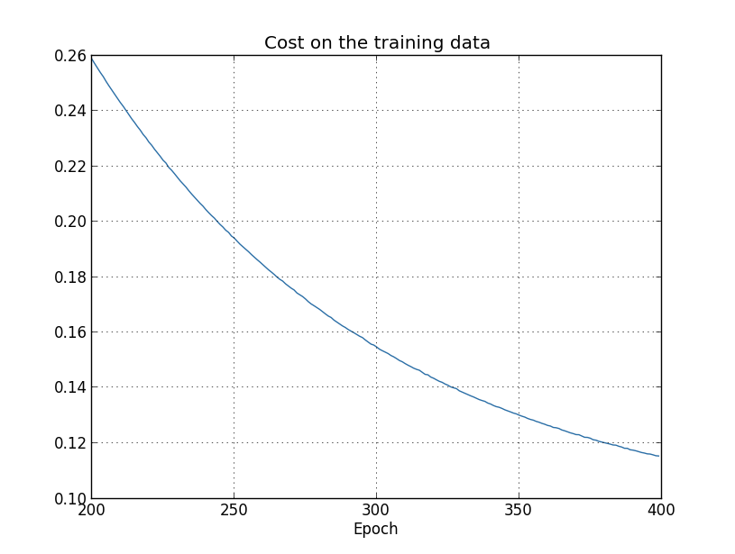
  Using the results we can plot the way the cost changes as the networklearns**This and the next four graphs were generated by the program overfitting.py.:

  

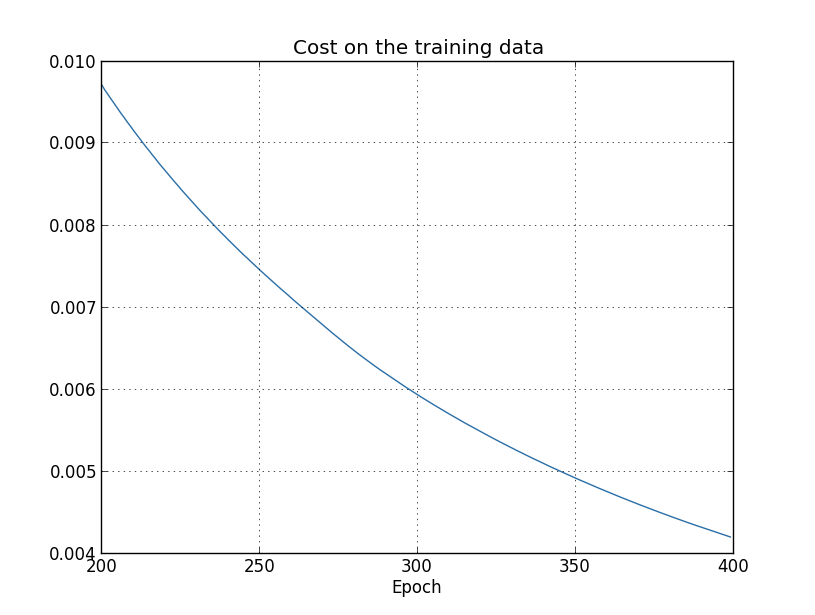
  This looks encouraging, showing a smooth decrease in the cost, just aswe expect. Note that I've only shown training epochs 200 through 399.This gives us a nice up-close view of the later stages of learning,which, as we'll see, turns out to be where the interesting action is.

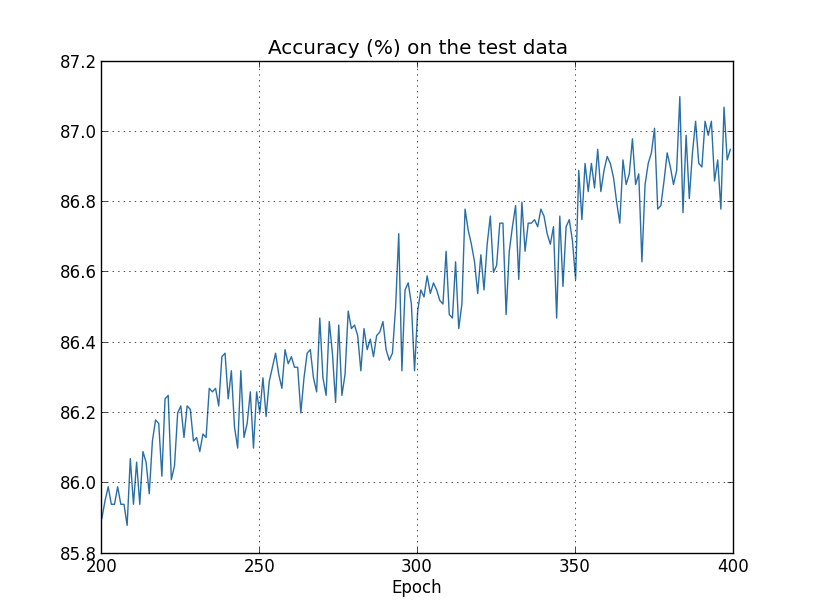
  Let's now look at how the classification accuracy on the test datachanges over time:

  

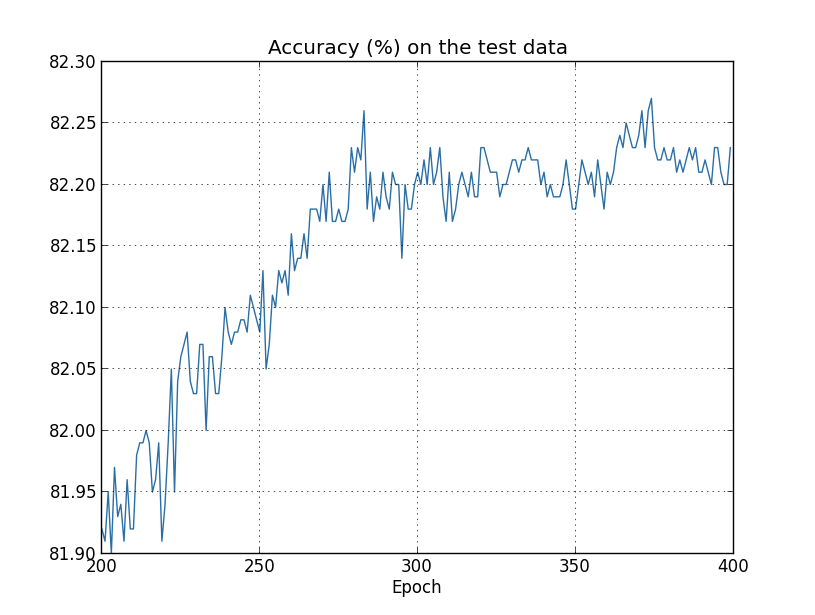
  Again, I've zoomed in quite a bit. In the first 200 epochs (notshown) the accuracy rises to just under 82 percent. The learning thengradually slows down. Finally, at around epoch 280 the classificationaccuracy pretty much stops improving. Later epochs merely see smallstochastic fluctuations near the value of the accuracy at epoch 280.Contrast this with the earlier graph, where the cost associated to thetraining data continues to smoothly drop. If we just look at thatcost, it appears that our model is still getting "better". But thetest accuracy results show the improvement is an illusion. Just likethe model that Fermi disliked, what our network learns after epoch 280no longer generalizes to the test data. And so it's not usefullearning. We say the network is overfitting orovertraining beyond epoch 280.

  You might wonder if the problem here is that I'm looking at thecost on the training data, as opposed to theclassification accuracy on the test data. In other words,maybe the problem is that we're making an apples and orangescomparison. What would happen if we compared the cost on the trainingdata with the cost on the test data, so we're comparing similarmeasures? Or perhaps we could compare the classification accuracy onboth the training data and the test data? In fact, essentially thesame phenomenon shows up no matter how we do the comparison. Thedetails do change, however. For instance, let's look at the cost onthe test data:

  

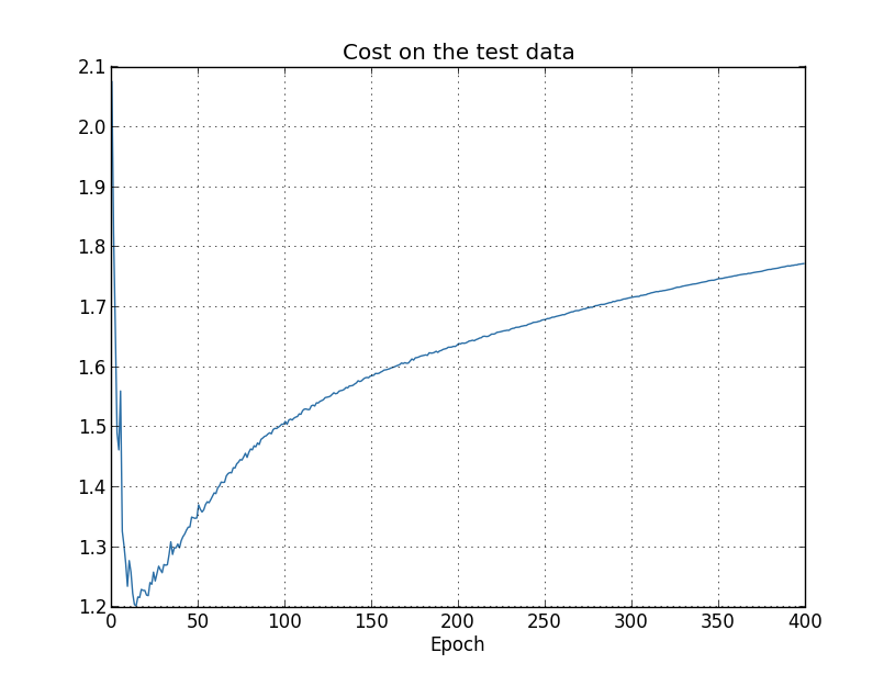
  We can see that the cost on the test data improves until around epoch15, but after that it actually starts to get worse, even though thecost on the training data is continuing to get better. This isanother sign that our model is overfitting. It poses a puzzle,though, which is whether we should regard epoch 15 or epoch 280 as thepoint at which overfitting is coming to dominate learning? From apractical point of view, what we really care about is improvingclassification accuracy on the test data, while the cost on the testdata is no more than a proxy for classification accuracy. And so itmakes most sense to regard epoch 280 as the point beyond whichoverfitting is dominating learning in our neural network.

  Another sign of overfitting may be seen in the classification accuracyon the training data:

  

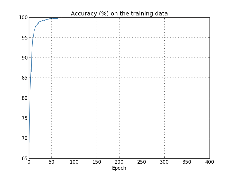
  The accuracy rises all the way up to 100

  percent. That is, ournetwork correctly classifies all 1,000 training images! Meanwhile,our test accuracy tops out at just 82.27

  percent. So our networkreally is learning about peculiarities of the training set, not justrecognizing digits in general. It's almost as though our network ismerely memorizing the training set, without understanding digits wellenough to generalize to the test set.

  Overfitting is a major problem in neural networks. This is especiallytrue in modern networks, which often have very large numbers ofweights and biases. To train effectively, we need a way of detectingwhen overfitting is going on, so we don't overtrain. And we'd like tohave techniques for reducing the effects of overfitting.

  The obvious way to detect overfitting is to use the approach above,keeping track of accuracy on the test data as our network trains. Ifwe see that the accuracy on the test data is no longer improving, thenwe should stop training. Of course, strictly speaking, this is notnecessarily a sign of overfitting. It might be that accuracy on thetest data and the training data both stop improving at the same time.Still, adopting this strategy will prevent overfitting.

  In fact, we'll use a variation on this strategy. Recall that when weload in the MNIST data we load in three data sets:

   
  >>> import mnist_loader 
  >>> training_data, validation_data, test_data = \
  ... mnist_loader.load_data_wrapper()
  

  Up to now we've been using the training_data andtest_data, and ignoring the validation_data. Thevalidation_data contains 10,000 images of digits, imageswhich are different from the 50,000 images in the MNIST trainingset, and the 10,000 images in the MNIST test set. Instead of usingthe test_data to prevent overfitting, we will use thevalidation_data. To do this, we'll use much the same strategyas was described above for the test_data. That is, we'llcompute the classification accuracy on the validation_data atthe end of each epoch. Once the classification accuracy on thevalidation_data has saturated, we stop training. This strategyis called early stopping. Of course, in practice we won'timmediately know when the accuracy has saturated. Instead, wecontinue training until we're confident that the accuracy hassaturated**It requires some judgment to determine when to stop. In my earlier graphs I identified epoch 280 as the place at which accuracy saturated. It's possible that was too pessimistic. Neural networks sometimes plateau for a while in training, before continuing to improve. I wouldn't be surprised if more learning could have occurred even after epoch 400, although the magnitude of any further improvement would likely be small. So it's possible to adopt more or less aggressive strategies for early stopping..

  Why use the validation_data to prevent overfitting, rather thanthe test_data? In fact, this is part of a more generalstrategy, which is to use the validation_data to evaluatedifferent trial choices of hyper-parameters such as the number ofepochs to train for, the learning rate, the best network architecture,and so on. We use such evaluations to find and set good values forthe hyper-parameters. Indeed, although I haven't mentioned it untilnow, that is, in part, how I arrived at the hyper-parameter choicesmade earlier in this book. (More on thislater.)

  Of course, that doesn't in any way answer the question of why we'reusing the validation_data to prevent overfitting, rather thanthe test_data. Instead, it replaces it with a more generalquestion, which is why we're using the validation_data ratherthan the test_data to set good hyper-parameters? To understandwhy, consider that when setting hyper-parameters we're likely to trymany different choices for the hyper-parameters. If we set thehyper-parameters based on evaluations of the test_data it'spossible we'll end up overfitting our hyper-parameters to thetest_data. That is, we may end up finding hyper-parameterswhich fit particular peculiarities of the test_data, but wherethe performance of the network won't generalize to other data sets.We guard against that by figuring out the hyper-parameters using thevalidation_data. Then, once we've got the hyper-parameters wewant, we do a final evaluation of accuracy using the test_data.That gives us confidence that our results on the test_data area true measure of how well our neural network generalizes. To put itanother way, you can think of the validation data as a type oftraining data that helps us learn good hyper-parameters. Thisapproach to finding good hyper-parameters is sometimes known as thehold out method, since the validation_data is kept apartor "held out" from the training_data.

  Now, in practice, even after evaluating performance on thetest_data we may change our minds and want to try anotherapproach - perhaps a different network architecture - which willinvolve finding a new set of hyper-parameters. If we do this, isn'tthere a danger we'll end up overfitting to the test_data aswell? Do we need a potentially infinite regress of data sets, so wecan be confident our results will generalize? Addressing this concernfully is a deep and difficult problem. But for our practicalpurposes, we're not going to worry too much about this question.Instead, we'll plunge ahead, using the basic hold out method, based onthe training_data, validation_data, andtest_data, as described above.

  We've been looking so far at overfitting when we're just using 1,000training images. What happens when we use the full training set of50,000 images? We'll keep all the other parameters the same (30hidden neurons, learning rate 0.5, mini-batch size of 10), but trainusing all 50,000 images for 30 epochs. Here's a graph showing theresults for the classification accuracy on both the training data andthe test data. Note that I've used the test data here, rather thanthe validation data, in order to make the results more directlycomparable with the earlier graphs.

  

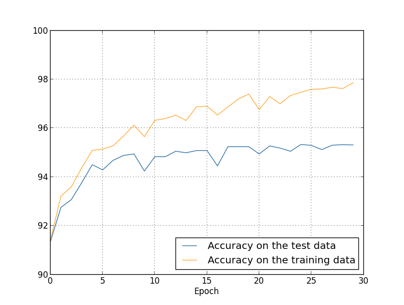
  As you can see, the accuracy on the test and training data remain muchcloser together than when we were using 1,000 training examples. Inparticular, the best classification accuracy of 97.86

  percent on thetraining data is only 1.53 percent higher than the 95.33 percenton the test data. That's compared to the 17.73

  percent gap we hadearlier! Overfitting is still going on, but it's been greatlyreduced. Our network is generalizing much better from the trainingdata to the test data. In general, one of the best ways of reducingoverfitting is to increase the size of the training data. With enoughtraining data it is difficult for even a very large network tooverfit. Unfortunately, training data can be expensive or difficultto acquire, so this is not always a practical option.

  Regularization

  Increasing the amount of training data is one way of reducingoverfitting. Are there other ways we can reduce the extent to whichoverfitting occurs? One possible approach is to reduce the size ofour network. However, large networks have the potential to be morepowerful than small networks, and so this is an option we'd only adoptreluctantly.

  Fortunately, there are other techniques which can reduce overfitting,even when we have a fixed network and fixed training data. These areknown as regularization techniques. In this section I describeone of the most commonly used regularization techniques, a techniquesometimes known as weight decay or L2 regularization.The idea of L2 regularization is to add an extra term to the costfunction, a term called the regularization term. Here's theregularized cross-entropy:

  C=−1n∑xj[yjlnaLj+(1−yj)ln(1−aLj)]+λ2n∑ww2.(85)

  The first term is just the usual expression for the cross-entropy.But we've added a second term, namely the sum of the squares of allthe weights in the network. This is scaled by a factor λ/2n

  , where λ>0 is known as the regularization parameter, and n is, as usual, the size of our training set.I'll discuss later how λ

  is chosen. It's also worth notingthat the regularization term doesn't include the biases. I'llalso come back to that below.

  Of course, it's possible to regularize other cost functions, such asthe quadratic cost. This can be done in a similar way:

  C=12n∑x∥y−aL∥2+λ2n∑ww2.(86)

  In both cases we can write the regularized cost function as

  C=C0+λ2n∑ww2,(87)
  where C0

  is the original, unregularized costfunction.

  Intuitively, the effect of regularization is to make it so the networkprefers to learn small weights, all other things being equal. Largeweights will only be allowed if they considerably improve the firstpart of the cost function. Put another way, regularization can beviewed as a way of compromising between finding small weights andminimizing the original cost function. The relative importance of thetwo elements of the compromise depends on the value of λ

  : when λ is small we prefer to minimize the original cost function,but when λ

  is large we prefer small weights.

  Now, it's really not at all obvious why making this kind of compromiseshould help reduce overfitting! But it turns out that it does. We'lladdress the question of why it helps in the next section. But first,let's work through an example showing that regularization really doesreduce overfitting.

  To construct such an example, we first need to figure out how to applyour stochastic gradient descent learning algorithm in a regularizedneural network. In particular, we need to know how to compute thepartial derivatives ∂C/∂w

  and ∂C/∂b

  for all the weights and biases in the network. Takingthe partial derivatives of Equation (87) gives

  ∂C∂w∂C∂b==∂C0∂w+λnw∂C0∂b.(88)(89)

  The ∂C0/∂w

  and ∂C0/∂b termscan be computed using backpropagation, as described inthe last chapter. And so we see that it's easy tocompute the gradient of the regularized cost function: just usebackpropagation, as usual, and then add λnw

  to thepartial derivative of all the weight terms. The partial derivativeswith respect to the biases are unchanged, and so the gradient descentlearning rule for the biases doesn't change from the usual rule:

  b→b−η∂C0∂b.(90)

  The learning rule for the weights becomes:

  w→=w−η∂C0∂w−ηλnw(1−ηλn)w−η∂C0∂w.(91)(92)

  This is exactly the same as the usual gradient descent learning rule,except we first rescale the weight w

  by a factor 1−ηλn

  . This rescaling is sometimes referred to asweight decay, since it makes the weights smaller. At firstglance it looks as though this means the weights are being drivenunstoppably toward zero. But that's not right, since the other termmay lead the weights to increase, if so doing causes a decrease in theunregularized cost function.

  Okay, that's how gradient descent works. What about stochasticgradient descent? Well, just as in unregularized stochastic gradientdescent, we can estimate ∂C0/∂w

  by averaging overa mini-batch of m

  training examples. Thus the regularized learningrule for stochastic gradient descent becomes(c.f. Equation (20))

  w→(1−ηλn)w−ηm∑x∂Cx∂w,(93)

  where the sum is over training examples x

  in the mini-batch, and Cx is the (unregularized) cost for each training example. This isexactly the same as the usual rule for stochastic gradient descent,except for the 1−ηλn

  weight decay factor.Finally, and for completeness, let me state the regularized learningrule for the biases. This is, of course, exactly the same as in theunregularized case (c.f. Equation (21)),

  b→b−ηm∑x∂Cx∂b,(94)
  where the sum is over training examples x

  in the mini-batch.

  Let's see how regularization changes the performance of our neuralnetwork. We'll use a network with 30

  hidden neurons, a mini-batchsize of 10 , a learning rate of 0.5 , and the cross-entropy costfunction. However, this time we'll use a regularization parameter of λ=0.1

  . Note that in the code, we use the variable namelmbda, because lambda is a reserved word in Python, withan unrelated meaning. I've also used the test_data again, notthe validation_data. Strictly speaking, we should use thevalidation_data, for all the reasons we discussed earlier. ButI decided to use the test_data because it makes the resultsmore directly comparable with our earlier, unregularized results. Youcan easily change the code to use the validation_data instead,and you'll find that it gives similar results.

   
  >>> import mnist_loader 
  >>> training_data, validation_data, test_data = \
  ... mnist_loader.load_data_wrapper() 
  >>> import network2 
  >>> net = network2.Network([784, 30, 10], cost=network2.CrossEntropyCost)
  >>> net.large_weight_initializer()
  >>> net.SGD(training_data[:1000], 400, 10, 0.5,
  ... evaluation_data=test_data, lmbda = 0.1,
  ... monitor_evaluation_cost=True, monitor_evaluation_accuracy=True,
  ... monitor_training_cost=True, monitor_training_accuracy=True)
  

  The cost on the training data decreases over the whole time, much asit did in the earlier, unregularized case**This and the next two graphs were produced with the program overfitting.py.:

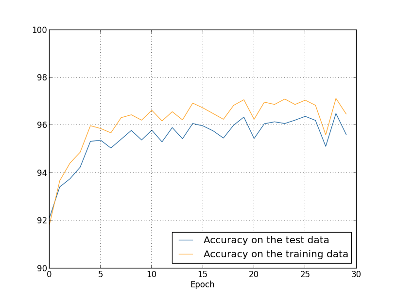
  But this time the accuracy on the test_data continues toincrease for the entire 400 epochs:

  

  Clearly, the use of regularization has suppressed overfitting. What'smore, the accuracy is considerably higher, with a peak classificationaccuracy of 87.1

  percent, compared to the peak of 82.27

  percentobtained in the unregularized case. Indeed, we could almost certainlyget considerably better results by continuing to train past 400epochs. It seems that, empirically, regularization is causing ournetwork to generalize better, and considerably reducing the effects ofoverfitting.

  What happens if we move out of the artificial environment of justhaving 1,000 training images, and return to the full 50,000 imagetraining set? Of course, we've seen already that overfitting is muchless of a problem with the full 50,000 images. Does regularizationhelp any further? Let's keep the hyper-parameters the same as before- 30

  epochs, learning rate 0.5 , mini-batch size of 10 .However, we need to modify the regularization parameter. The reasonis because the size n of the training set has changed from n=1,000 to n=50,000 , and this changes the weight decay factor 1−ηλn . If we continued to use λ=0.1 thatwould mean much less weight decay, and thus much less of aregularization effect. We compensate by changing to λ=5.0

  .

  Okay, let's train our network, stopping first to re-initialize theweights:

   
  >>> net.large_weight_initializer()
  >>> net.SGD(training_data, 30, 10, 0.5,
  ... evaluation_data=test_data, lmbda = 5.0,
  ... monitor_evaluation_accuracy=True, monitor_training_accuracy=True)
  

  We obtain the results:

  There's lots of good news here. First, our classification accuracy onthe test data is up, from 95.49

  percent when running unregularized,to 96.49

  percent. That's a big improvement. Second, we can seethat the gap between results on the training and test data is muchnarrower than before, running at under a percent. That's still asignificant gap, but we've obviously made substantial progressreducing overfitting.

  Finally, let's see what test classification accuracy we get when weuse 100 hidden neurons and a regularization parameter of λ=5.0

  . I won't go through a detailed analysis of overfitting here, thisis purely for fun, just to see how high an accuracy we can get when weuse our new tricks: the cross-entropy cost function and L2regularization.

   
  >>> net = network2.Network([784, 100, 10], cost=network2.CrossEntropyCost)
  >>> net.large_weight_initializer()
  >>> net.SGD(training_data, 30, 10, 0.5, lmbda=5.0,
  ... evaluation_data=validation_data,
  ... monitor_evaluation_accuracy=True)
  

  The final result is a classification accuracy of 97.92

  percent onthe validation data. That's a big jump from the 30 hidden neuroncase. In fact, tuning justa little more, to run for 60 epochs at η=0.1 and λ=5.0 we break the 98 percent barrier, achieving 98.04

  percentclassification accuracy on the validation data. Not bad for whatturns out to be 152 lines of code!

  I've described regularization as a way to reduce overfitting and toincrease classification accuracies. In fact, that's not the onlybenefit. Empirically, when doing multiple runs of our MNIST networks,but with different (random) weight initializations, I've found thatthe unregularized runs will occasionally get "stuck", apparentlycaught in local minima of the cost function. The result is thatdifferent runs sometimes provide quite different results. Bycontrast, the regularized runs have provided much more easilyreplicable results.

  Why is this going on? Heuristically, if the cost function isunregularized, then the length of the weight vector is likely to grow,all other things being equal. Over time this can lead to the weightvector being very large indeed. This can cause the weight vector toget stuck pointing in more or less the same direction, since changesdue to gradient descent only make tiny changes to the direction, whenthe length is long. I believe this phenomenon is making it hard forour learning algorithm to properly explore the weight space, andconsequently harder to find good minima of the cost function.

  Why does regularization help reduce overfitting?

  We've seen empirically that regularization helps reduce overfitting.That's encouraging but, unfortunately, it's not obvious whyregularization helps! A standard story people tell to explain what'sgoing on is along the following lines: smaller weights are, in somesense, lower complexity, and so provide a simpler and more powerfulexplanation for the data, and should thus be preferred. That's apretty terse story, though, and contains several elements that perhapsseem dubious or mystifying. Let's unpack the story and examine itcritically. To do that, let's suppose we have a simple data set forwhich we wish to build a model:

  012345x012345678910y

  Implicitly, we're studying some real-world phenomenon here, with x

  and y representing real-world data. Our goal is to build a modelwhich lets us predict y as a function of x . We could try usingneural networks to build such a model, but I'm going to do somethingeven simpler: I'll try to model y as a polynomial in x . I'm doingthis instead of using neural nets because using polynomials will makethings particularly transparent. Once we've understood the polynomialcase, we'll translate to neural networks. Now, there are ten pointsin the graph above, which means we can find a unique 9 th-orderpolynomial y=a0x9+a1x8+…+a9

  which fits the dataexactly. Here's the graph of that polynomial**I won't show the coefficients explicitly, although they are easy to find using a routine such as Numpy's polyfit. You can view the exact form of the polynomial in the source code for the graph if you're curious. It's the function p(x) defined starting on line 14 of the program which produces the graph.:

  012345x012345678910y

  That provides an exact fit. But we can also get a good fit using thelinear model y=2x

  :

  012345x012345678910y

  Which of these is the better model? Which is more likely to be true?And which model is more likely to generalize well to other examples ofthe same underlying real-world phenomenon?

  These are difficult questions. In fact, we can't determine withcertainty the answer to any of the above questions, without much moreinformation about the underlying real-world phenomenon. But let'sconsider two possibilities: (1) the 9

  th order polynomial is, infact, the model which truly describes the real-world phenomenon, andthe model will therefore generalize perfectly; (2) the correct modelis y=2x

  , but there's a little additional noise due to, say,measurement error, and that's why the model isn't an exact fit.

  It's not a priori possible to say which of these twopossibilities is correct. (Or, indeed, if some third possibilityholds). Logically, either could be true. And it's not a trivialdifference. It's true that on the data provided there's only a smalldifference between the two models. But suppose we want to predict thevalue of y

  corresponding to some large value of x , much largerthan any shown on the graph above. If we try to do that there will bea dramatic difference between the predictions of the two models, asthe 9 th order polynomial model comes to be dominated by the x9

  term, while the linear model remains, well, linear.

  One point of view is to say that in science we should go with thesimpler explanation, unless compelled not to. When we find a simplemodel that seems to explain many data points we are tempted to shout"Eureka!" After all, it seems unlikely that a simple explanationshould occur merely by coincidence. Rather, we suspect that the modelmust be expressing some underlying truth about the phenomenon. In thecase at hand, the model y=2x+noise

  seems much simpler than y=a0x9+a1x8+… . It would be surprising if thatsimplicity had occurred by chance, and so we suspect that y=2x+noise

  expresses some underlying truth. In this point of view, the9th order model is really just learning the effects of localnoise. And so while the 9th order model works perfectly for theseparticular data points, the model will fail to generalize to otherdata points, and the noisy linear model will have greater predictivepower.

  Let's see what this point of view means for neural networks. Supposeour network mostly has small weights, as will tend to happen in aregularized network. The smallness of the weights means that thebehaviour of the network won't change too much if we change a fewrandom inputs here and there. That makes it difficult for aregularized network to learn the effects of local noise in the data.Think of it as a way of making it so single pieces of evidence don'tmatter too much to the output of the network. Instead, a regularizednetwork learns to respond to types of evidence which are seen oftenacross the training set. By contrast, a network with large weightsmay change its behaviour quite a bit in response to small changes inthe input. And so an unregularized network can use large weights tolearn a complex model that carries a lot of information about thenoise in the training data. In a nutshell, regularized networks areconstrained to build relatively simple models based on patterns seenoften in the training data, and are resistant to learningpeculiarities of the noise in the training data. The hope is thatthis will force our networks to do real learning about the phenomenonat hand, and to generalize better from what they learn.

  With that said, this idea of preferring simpler explanation shouldmake you nervous. People sometimes refer to this idea as "Occam'sRazor", and will zealously apply it as though it has the status ofsome general scientific principle. But, of course, it's not a generalscientific principle. There is no a priori logical reason toprefer simple explanations over more complex explanations. Indeed,sometimes the more complex explanation turns out to be correct.

  Let me describe two examples where more complex explanations haveturned out to be correct. In the 1940s the physicist Marcel Scheinannounced the discovery of a new particle of nature. The company heworked for, General Electric, was ecstatic, and publicized thediscovery widely. But the physicist Hans Bethe was skeptical. Bethevisited Schein, and looked at the plates showing the tracks ofSchein's new particle. Schein showed Bethe plate after plate, but oneach plate Bethe identified some problem that suggested the datashould be discarded. Finally, Schein showed Bethe a plate that lookedgood. Bethe said it might just be a statistical fluke. Schein:"Yes, but the chance that this would be statistics, even according toyour own formula, is one in five." Bethe: "But we have alreadylooked at five plates." Finally, Schein said: "But on my plates,each one of the good plates, each one of the good pictures, youexplain by a different theory, whereas I have one hypothesis thatexplains all the plates, that they are [the new particle]." Bethereplied: "The sole difference between your and my explanations isthat yours is wrong and all of mine are right. Your singleexplanation is wrong, and all of my multiple explanations are right."Subsequent work confirmed that Nature agreed with Bethe, and Schein'sparticle is no more**The story is related by the physicist Richard Feynman in an interview with the historian Charles Weiner..

  As a second example, in 1859 the astronomer Urbain Le Verrier observedthat the orbit of the planet Mercury doesn't have quite the shape thatNewton's theory of gravitation says it should have. It was a tiny,tiny deviation from Newton's theory, and several of the explanationsproferred at the time boiled down to saying that Newton's theory wasmore or less right, but needed a tiny alteration. In 1916, Einsteinshowed that the deviation could be explained very well using hisgeneral theory of relativity, a theory radically different toNewtonian gravitation, and based on much more complex mathematics.Despite that additional complexity, today it's accepted thatEinstein's explanation is correct, and Newtonian gravity, even in itsmodified forms, is wrong. This is in part because we now know thatEinstein's theory explains many other phenomena which Newton's theoryhas difficulty with. Furthermore, and even more impressively,Einstein's theory accurately predicts several phenomena which aren'tpredicted by Newtonian gravity at all. But these impressive qualitiesweren't entirely obvious in the early days. If one had judged merelyon the grounds of simplicity, then some modified form of Newton'stheory would arguably have been more attractive.

  There are three morals to draw from these stories. First, it can bequite a subtle business deciding which of two explanations is truly"simpler". Second, even if we can make such a judgment, simplicityis a guide that must be used with great caution! Third, the true testof a model is not simplicity, but rather how well it does inpredicting new phenomena, in new regimes of behaviour.

  With that said, and keeping the need for caution in mind, it's anempirical fact that regularized neural networks usually generalizebetter than unregularized networks. And so through the remainder ofthe book we will make frequent use of regularization. I've includedthe stories above merely to help convey why no-one has yet developedan entirely convincing theoretical explanation for why regularizationhelps networks generalize. Indeed, researchers continue to writepapers where they try different approaches to regularization, comparethem to see which works better, and attempt to understand why differentapproaches work better or worse. And so you can view regularizationas something of a kludge. While it often helps, we don't have anentirely satisfactory systematic understanding of what's going on,merely incomplete heuristics and rules of thumb.

  There's a deeper set of issues here, issues which go to the heart ofscience. It's the question of how we generalize. Regularization maygive us a computational magic wand that helps our networks generalizebetter, but it doesn't give us a principled understanding of howgeneralization works, nor of what the best approach is**These issues go back to the problem of induction, famously discussed by the Scottish philosopher David Hume in "An Enquiry Concerning Human Understanding" (1748). The problem of induction has been given a modern machine learning form in the no-free lunch theorem (link) of David Wolpert and William Macready (1997)..

  This is particularly galling because in everyday life, we humansgeneralize phenomenally well. Shown just a few images of an elephanta child will quickly learn to recognize other elephants. Of course,they may occasionally make mistakes, perhaps confusing a rhinocerosfor an elephant, but in general this process works remarkablyaccurately. So we have a system - the human brain - with a hugenumber of free parameters. And after being shown just one or a fewtraining images that system learns to generalize to other images. Ourbrains are, in some sense, regularizing amazingly well! How do we doit? At this point we don't know. I expect that in years to come wewill develop more powerful techniques for regularization in artificialneural networks, techniques that will ultimately enable neural nets togeneralize well even from small data sets.

  In fact, our networks already generalize better than one might a priori expect. A network with 100 hidden neurons has nearly 80,000parameters. We have only 50,000 images in our training data. It'slike trying to fit an 80,000th degree polynomial to 50,000 datapoints. By all rights, our network should overfit terribly. And yet,as we saw earlier, such a network actually does a pretty good jobgeneralizing. Why is that the case? It's not well understood. Ithas been conjectured**In Gradient-Based Learning Applied to Document Recognition, by Yann LeCun, Léon Bottou, Yoshua Bengio, and Patrick Haffner (1998). that "the dynamics of gradient descent learning inmultilayer nets has a `self-regularization' effect". This isexceptionally fortunate, but it's also somewhat disquieting that wedon't understand why it's the case. In the meantime, we will adoptthe pragmatic approach and use regularization whenever we can. Ourneural networks will be the better for it.

  Let me conclude this section by returning to a detail which I leftunexplained earlier: the fact that L2 regularization doesn'tconstrain the biases. Of course, it would be easy to modify theregularization procedure to regularize the biases. Empirically, doingthis often doesn't change the results very much, so to some extentit's merely a convention whether to regularize the biases or not.However, it's worth noting that having a large bias doesn't make aneuron sensitive to its inputs in the same way as having largeweights. And so we don't need to worry about large biases enablingour network to learn the noise in our training data. At the sametime, allowing large biases gives our networks more flexibility inbehaviour - in particular, large biases make it easier for neuronsto saturate, which is sometimes desirable. For these reasons we don'tusually include bias terms when regularizing.

  Other techniques for regularization

  There are many regularization techniques other than L2 regularization.In fact, so many techniques have been developed that I can't possiblysummarize them all. In this section I briefly describe three otherapproaches to reducing overfitting: L1 regularization, dropout, andartificially increasing the training set size. We won't go intonearly as much depth studying these techniques as we did earlier.Instead, the purpose is to get familiar with the main ideas, and toappreciate something of the diversity of regularization techniquesavailable.

  L1 regularization: In this approach we modify theunregularized cost function by adding the sum of the absolute valuesof the weights:

  C=C0+λn∑w|w|.(95)

  Intuitively, this is similar to L2 regularization, penalizing largeweights, and tending to make the network prefer small weights. Ofcourse, the L1 regularization term isn't the same as the L2regularization term, and so we shouldn't expect to get exactly thesame behaviour. Let's try to understand how the behaviour of anetwork trained using L1 regularization differs from a network trainedusing L2 regularization.

  To do that, we'll look at the partial derivatives of the costfunction. Differentiating (95) we obtain:

  ∂C∂w=∂C0∂w+λnsgn(w),(96)

  where sgn(w)

  is the sign of w , that is, +1 if w ispositive, and −1 if w is negative. Using this expression, we caneasily modify backpropagation to do stochastic gradient descent usingL1 regularization. The resulting update rule for an L1 regularizednetwork is
  w→w′=w−ηλnsgn(w)−η∂C0∂w,(97)

  where, as per usual, we can estimate ∂C0/∂w

  usinga mini-batch average, if we wish. Compare that to the update rule forL2 regularization (c.f. Equation (93)),
  w→w′=w(1−ηλn)−η∂C0∂w.(98)
  In both expressions the effect of regularization is to shrink theweights. This accords with our intuition that both kinds ofregularization penalize large weights. But the way the weights shrinkis different. In L1 regularization, the weights shrink by a constantamount toward 0 . In L2 regularization, the weights shrink by anamount which is proportional to w . And so when a particular weighthas a large magnitude, |w| , L1 regularization shrinks the weightmuch less than L2 regularization does. By contrast, when |w|

  issmall, L1 regularization shrinks the weight much more than L2regularization. The net result is that L1 regularization tends toconcentrate the weight of the network in a relatively small number ofhigh-importance connections, while the other weights are driven towardzero.

  I've glossed over an issue in the above discussion, which is that thepartial derivative ∂C/∂w

  isn't defined when w=0 . The reason is that the function |w| has a sharp "corner" at w=0 , and so isn't differentiable at that point. That's okay,though. What we'll do is just apply the usual (unregularized) rulefor stochastic gradient descent when w=0 . That should be okay -intuitively, the effect of regularization is to shrink weights, andobviously it can't shrink a weight which is already 0 . To put itmore precisely, we'll use Equations (96)and (97) with the convention that sgn(0)=0

  .That gives a nice, compact rule for doing stochastic gradient descentwith L1 regularization.

  Dropout: Dropout is a radically different technique forregularization. Unlike L1 and L2 regularization, dropout doesn't relyon modifying the cost function. Instead, in dropout we modify thenetwork itself. Let me describe the basic mechanics of how dropoutworks, before getting into why it works, and what the results are.

  Suppose we're trying to train a network:

  

  In particular, suppose we have a training input x

  and correspondingdesired output y . Ordinarily, we'd train by forward-propagating x

  through the network, and then backpropagating to determine thecontribution to the gradient. With dropout, this process is modified.We start by randomly (and temporarily) deleting half the hiddenneurons in the network, while leaving the input and output neuronsuntouched. After doing this, we'll end up with a network along thefollowing lines. Note that the dropout neurons, i.e., the neuronswhich have been temporarily deleted, are still ghosted in:

  

  We forward-propagate the input x

  through the modified network, andthen backpropagate the result, also through the modified network.After doing this over a mini-batch of examples, we update theappropriate weights and biases. We then repeat the process, firstrestoring the dropout neurons, then choosing a new random subset ofhidden neurons to delete, estimating the gradient for a differentmini-batch, and updating the weights and biases in the network.

  By repeating this process over and over, our network will learn a setof weights and biases. Of course, those weights and biases will havebeen learnt under conditions in which half the hidden neurons weredropped out. When we actually run the full network that means thattwice as many hidden neurons will be active. To compensate for that,we halve the weights outgoing from the hidden neurons.

  This dropout procedure may seem strange and ad hoc. Why wouldwe expect it to help with regularization? To explain what's going on,I'd like you to briefly stop thinking about dropout, and insteadimagine training neural networks in the standard way (no dropout). Inparticular, imagine we train several different neural networks, allusing the same training data. Of course, the networks may not startout identical, and as a result after training they may sometimes givedifferent results. When that happens we could use some kind ofaveraging or voting scheme to decide which output to accept. Forinstance, if we have trained five networks, and three of them areclassifying a digit as a "3", then it probably really is a "3".The other two networks are probably just making a mistake. This kindof averaging scheme is often found to be a powerful (though expensive)way of reducing overfitting. The reason is that the differentnetworks may overfit in different ways, and averaging may helpeliminate that kind of overfitting.

  What's this got to do with dropout? Heuristically, when we dropoutdifferent sets of neurons, it's rather like we're training differentneural networks. And so the dropout procedure is like averaging theeffects of a very large number of different networks. The differentnetworks will overfit in different ways, and so, hopefully, the neteffect of dropout will be to reduce overfitting.

  A related heuristic explanation for dropout is given in one of theearliest papers to use thetechnique**ImageNet Classification with Deep Convolutional Neural Networks, by Alex Krizhevsky, Ilya Sutskever, and Geoffrey Hinton (2012).: "Thistechnique reduces complex co-adaptations of neurons, since a neuroncannot rely on the presence of particular other neurons. It is,therefore, forced to learn more robust features that are useful inconjunction with many different random subsets of the other neurons."In other words, if we think of our network as a model which is makingpredictions, then we can think of dropout as a way of making sure thatthe model is robust to the loss of any individual piece of evidence.In this, it's somewhat similar to L1 and L2 regularization, which tendto reduce weights, and thus make the network more robust to losing anyindividual connection in the network.

  Of course, the true measure of dropout is that it has been verysuccessful in improving the performance of neural networks. Theoriginalpaper**Improving neural networks by preventing co-adaptation of feature detectors by Geoffrey Hinton, Nitish Srivastava, Alex Krizhevsky, Ilya Sutskever, and Ruslan Salakhutdinov (2012). Note that the paper discusses a number of subtleties that I have glossed over in this brief introduction. introducing the technique applied it to manydifferent tasks. For us, it's of particular interest that they applieddropout to MNIST digit classification, using a vanilla feedforwardneural network along lines similar to those we've been considering.The paper noted that the best result anyone had achieved up to thatpoint using such an architecture was 98.4

  percent classificationaccuracy on the test set. They improved that to 98.7

  percentaccuracy using a combination of dropout and a modified form of L2regularization. Similarly impressive results have been obtained formany other tasks, including problems in image and speech recognition,and natural language processing. Dropout has been especially usefulin training large, deep networks, where the problem of overfitting isoften acute.

  Artificially expanding the training data: We saw earlier thatour MNIST classification accuracy dropped down to percentages in themid-80s when we used only 1,000 training images. It's not surprisingthat this is the case, since less training data means our network willbe exposed to fewer variations in the way human beings write digits.Let's try training our 30 hidden neuron network with a variety ofdifferent training data set sizes, to see how performance varies. Wetrain using a mini-batch size of 10, a learning rate η=0.5

  , aregularization parameter λ=5.0 , and the cross-entropy costfunction. We will train for 30 epochs when the full training data setis used, and scale up the number of epochs proportionally when smallertraining sets are used. To ensure the weight decay factor remains thesame across training sets, we will use a regularization parameter of λ=5.0 when the full training data set is used, and scaledown λ

  proportionally when smaller training sets areused**This and the next two graph are produced with the program more_data.py..

  

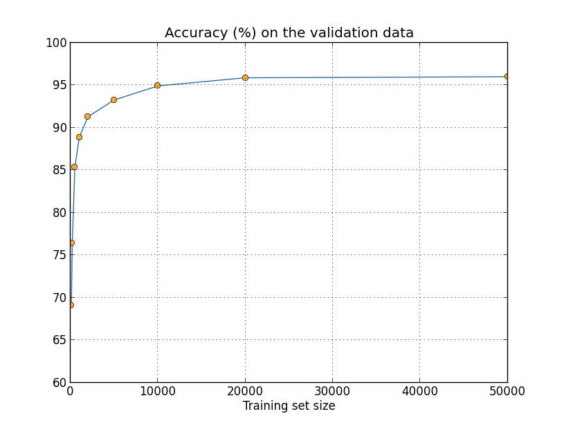
  As you can see, the classification accuracies improve considerably aswe use more training data. Presumably this improvement would continuestill further if more data was available. Of course, looking at thegraph above it does appear that we're getting near saturation.Suppose, however, that we redo the graph with the training set sizeplotted logarithmically:

  

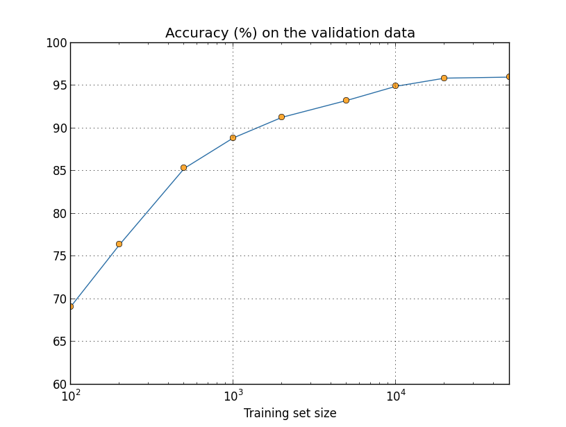
  It seems clear that the graph is still going up toward the end. Thissuggests that if we used vastly more training data - say, millionsor even billions of handwriting samples, instead of just 50,000 -then we'd likely get considerably better performance, even from thisvery small network.

  Obtaining more training data is a great idea. Unfortunately, it can beexpensive, and so is not always possible in practice. However,there's another idea which can work nearly as well, and that's toartificially expand the training data. Suppose, for example, that wetake an MNIST training image of a five,

  

  and rotate it by a small amount, let's say 15 degrees:

  

  It's still recognizably the same digit. And yet at the pixel levelit's quite different to any image currently in the MNIST trainingdata. It's conceivable that adding this image to the training datamight help our network learn more about how to classify digits.What's more, obviously we're not limited to adding just this oneimage. We can expand our training data by making many smallrotations of all the MNIST training images, and then using theexpanded training data to improve our network's performance.

  This idea is very powerful and has been widely used. Let's look atsome of the results from apaper**Best Practices for Convolutional Neural Networks Applied to Visual Document Analysis, by Patrice Simard, Dave Steinkraus, and John Platt (2003). which applied several variations of the idea toMNIST. One of the neural network architectures they considered wasalong similar lines to what we've been using, a feedforward networkwith 800 hidden neurons and using the cross-entropy cost function.Running the network with the standard MNIST training data theyachieved a classification accuracy of 98.4 percent on their test set.But then they expanded the training data, using not just rotations, asI described above, but also translating and skewing the images. Bytraining on the expanded data set they increased their network'saccuracy to 98.9 percent. They also experimented with what theycalled "elastic distortions", a special type of image distortionintended to emulate the random oscillations found in hand muscles. Byusing the elastic distortions to expand the data they achieved an evenhigher accuracy, 99.3 percent. Effectively, they were broadening theexperience of their network by exposing it to the sort of variationsthat are found in real handwriting.

  Variations on this idea can be used to improve performance on manylearning tasks, not just handwriting recognition. The generalprinciple is to expand the training data by applying operations thatreflect real-world variation. It's not difficult to think of ways ofdoing this. Suppose, for example, that you're building a neuralnetwork to do speech recognition. We humans can recognize speech evenin the presence of distortions such as background noise. And so youcan expand your data by adding background noise. We can alsorecognize speech if it's sped up or slowed down. So that's another waywe can expand the training data. These techniques are not always used- for instance, instead of expanding the training data by addingnoise, it may well be more efficient to clean up the input to thenetwork by first applying a noise reduction filter. Still, it's worthkeeping the idea of expanding the training data in mind, and lookingfor opportunities to apply it.

  Exercise

  • As discussed above, one way of expanding the MNIST training data is to use small rotations of training images. What's a problem that might occur if we allow arbitrarily large rotations of training images?

  An aside on big data and what it means to compare classification accuracies: Let's look again at how our neuralnetwork's accuracy varies with training set size:

  

  Suppose that instead of using a neural network we use some othermachine learning technique to classify digits. For instance, let'stry using the support vector machines (SVM) which we met briefly backin Chapter 1. As was the case in Chapter 1,don't worry if you're not familiar with SVMs, we don't need tounderstand their details. Instead, we'll use the SVM supplied by thescikit-learn library. Here'show SVM performance varies as a function of training set size. I'veplotted the neural net results as well, to make comparisoneasy**This graph was produced with the program more_data.py (as were the last few graphs).:

  

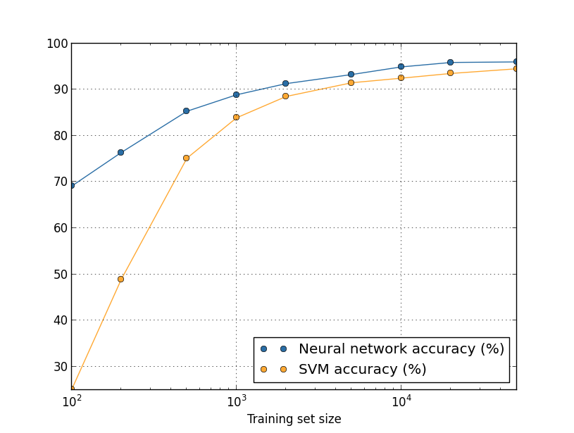
  Probably the first thing that strikes you about this graph is that ourneural network outperforms the SVM for every training set size.That's nice, although you shouldn't read too much into it, since Ijust used the out-of-the-box settings from scikit-learn's SVM, whilewe've done a fair bit of work improving our neural network. A moresubtle but more interesting fact about the graph is that if we trainour SVM using 50,000 images then it actually has better performance(94.48 percent accuracy) than our neural network does when trainedusing 5,000 images (93.24 percent accuracy). In other words, moretraining data can sometimes compensate for differences in the machinelearning algorithm used.

  Something even more interesting can occur. Suppose we're trying tosolve a problem using two machine learning algorithms, algorithm A andalgorithm B. It sometimes happens that algorithm A will outperformalgorithm B with one set of training data, while algorithm B willoutperform algorithm A with a different set of training data. Wedon't see that above - it would require the two graphs to cross -but it does happen**Striking examples may be found in Scaling to very very large corpora for natural language disambiguation, by Michele Banko and Eric Brill (2001).. The correct response to thequestion "Is algorithm A better than algorithm B?" is really: "Whattraining data set are you using?"

  All this is a caution to keep in mind, both when doing development,and when reading research papers. Many papers focus on finding newtricks to wring out improved performance on standard benchmark datasets. "Our whiz-bang technique gave us an improvement of X percenton standard benchmark Y" is a canonical form of research claim. Suchclaims are often genuinely interesting, but they must be understood asapplying only in the context of the specific training data set used.Imagine an alternate history in which the people who originallycreated the benchmark data set had a larger research grant. Theymight have used the extra money to collect more training data. It'sentirely possible that the "improvement" due to the whiz-bangtechnique would disappear on a larger data set. In other words, thepurported improvement might be just an accident of history. Themessage to take away, especially in practical applications, is thatwhat we want is both better algorithms and better trainingdata. It's fine to look for better algorithms, but make sure you'renot focusing on better algorithms to the exclusion of easy winsgetting more or better training data.

  Problem

  • (Research problem) How do our machine learning algorithms perform in the limit of very large data sets? For any given algorithm it's natural to attempt to define a notion of asymptotic performance in the limit of truly big data. A quick-and-dirty approach to this problem is to simply try fitting curves to graphs like those shown above, and then to extrapolate the fitted curves out to infinity. An objection to this approach is that different approaches to curve fitting will give different notions of asymptotic performance. Can you find a principled justification for fitting to some particular class of curves? If so, compare the asymptotic performance of several different machine learning algorithms.

  Summing up: We've now completed our dive into overfitting andregularization. Of course, we'll return again to the issue. As I'vementioned several times, overfitting is a major problem in neuralnetworks, especially as computers get more powerful, and we have theability to train larger networks. As a result there's a pressing needto develop powerful regularization techniques to reduce overfitting,and this is an extremely active area of current work.

  Weight initialization

  When we create our neural networks, we have to make choices for theinitial weights and biases. Up to now, we've been choosing themaccording to a prescription which I discussed only brieflyback in Chapter 1. Just toremind you, that prescription was to choose both the weights andbiases using independent Gaussian random variables, normalized to havemean 0

  and standard deviation 1

  . While this approach has workedwell, it was quite ad hoc, and it's worth revisiting to see ifwe can find a better way of setting our initial weights and biases,and perhaps help our neural networks learn faster.

  It turns out that we can do quite a bit better than initializing withnormalized Gaussians. To see why, suppose we're working with anetwork with a large number - say 1,000

  - of input neurons. Andlet's suppose we've used normalized Gaussians to initialize theweights connecting to the first hidden layer. For now I'm going toconcentrate specifically on the weights connecting the input neuronsto the first neuron in the hidden layer, and ignore the rest of thenetwork:

  

  We'll suppose for simplicity that we're trying to train using atraining input x

  in which half the input neurons are on, i.e., setto 1 , and half the input neurons are off, i.e., set to 0 . Theargument which follows applies more generally, but you'll get the gistfrom this special case. Let's consider the weighted sum z=∑jwjxj+b of inputs to our hidden neuron. 500 terms in this sumvanish, because the corresponding input xj is zero. And so z isa sum over a total of 501 normalized Gaussian random variables,accounting for the 500 weight terms and the 1 extra bias term.Thus z is itself distributed as a Gaussian with mean zero andstandard deviation 501−−−√≈22.4 . That is, z

  has a verybroad Gaussian distribution, not sharply peaked at all:

  -30-20-1001020300.02

  In particular, we can see from this graph that it's quite likely that |z|

  will be pretty large, i.e., either z≫1 or z≪−1 . Ifthat's the case then the output σ(z) from the hidden neuronwill be very close to either 1 or 0

  . That means our hidden neuronwill have saturated. And when that happens, as we know, making smallchanges in the weights will make only absolutely miniscule changes inthe activation of our hidden neuron. That miniscule change in theactivation of the hidden neuron will, in turn, barely affect the restof the neurons in the network at all, and we'll see a correspondinglyminiscule change in the cost function. As a result, those weightswill only learn very slowly when we use the gradient descentalgorithm**We discussed this in more detail in Chapter 2, where we used the equations of backpropagation to show that weights input to saturated neurons learned slowly.. It's similar to the problem we discussedearlier in this chapter, in which output neurons which saturated onthe wrong value caused learning to slow down. We addressed thatearlier problem with a clever choice of cost function. Unfortunately,while that helped with saturated output neurons, it does nothing atall for the problem with saturated hidden neurons.

  I've been talking about the weights input to the first hidden layer.Of course, similar arguments apply also to later hidden layers: if theweights in later hidden layers are initialized using normalizedGaussians, then activations will often be very close to 0

  or 1

  ,and learning will proceed very slowly.

  Is there some way we can choose better initializations for the weightsand biases, so that we don't get this kind of saturation, and so avoida learning slowdown? Suppose we have a neuron with nin

  inputweights. Then we shall initialize those weights as Gaussian randomvariables with mean 0 and standard deviation 1/nin−−−√ .That is, we'll squash the Gaussians down, making it less likely thatour neuron will saturate. We'll continue to choose the bias as aGaussian with mean 0 and standard deviation 1 , for reasons I'llreturn to in a moment. With these choices, the weighted sum z=∑jwjxj+b will again be a Gaussian random variable with mean 0 , but it'll be much more sharply peaked than it was before.Suppose, as we did earlier, that 500 of the inputs are zero and 500 are 1 . Then it's easy to show (see the exercise below) that z has a Gaussian distribution with mean 0 and standard deviation 3/2−−−√=1.22…

  . This is much more sharply peaked thanbefore, so much so that even the graph below understates thesituation, since I've had to rescale the vertical axis, when comparedto the earlier graph:

  -30-20-1001020300.4

  Such a neuron is much less likely to saturate, and correspondinglymuch less likely to have problems with a learning slowdown.

  Exercise

  • Verify that the standard deviation of z=∑jwjxj+b
  in the paragraph above is 3/2−−−√
  • . It may help to know that: (a) the variance of a sum of independent random variables is the sum of the variances of the individual random variables; and (b) the variance is the square of the standard deviation.

  I stated above that we'll continue to initialize the biases as before,as Gaussian random variables with a mean of 0

  and a standarddeviation of 1 . This is okay, because it doesn't make it too muchmore likely that our neurons will saturate. In fact, it doesn't muchmatter how we initialize the biases, provided we avoid the problemwith saturation. Some people go so far as to initialize all thebiases to 0

  , and rely on gradient descent to learn appropriatebiases. But since it's unlikely to make much difference, we'llcontinue with the same initialization procedure as before.

  Let's compare the results for both our old and new approaches toweight initialization, using the MNIST digit classification task. Asbefore, we'll use 30

  hidden neurons, a mini-batch size of 10 , aregularization parameter λ=5.0 , and the cross-entropy costfunction. We will decrease the learning rate slightly from η=0.5 to 0.1

  , since that makes the results a little more easilyvisible in the graphs. We can train using the old method of weightinitialization:

  >>> import mnist_loader
  >>> training_data, validation_data, test_data = \
  ... mnist_loader.load_data_wrapper()
  >>> import network2
  >>> net = network2.Network([784, 30, 10], cost=network2.CrossEntropyCost)
  >>> net.large_weight_initializer()
  >>> net.SGD(training_data, 30, 10, 0.1, lmbda = 5.0,
  ... evaluation_data=validation_data, 
  ... monitor_evaluation_accuracy=True)
  

  We can also train using the new approach to weight initialization.This is actually even easier, since network2's default way ofinitializing the weights is using this new approach. That means wecan omit the net.large_weight_initializer() call above:

  >>> net = network2.Network([784, 30, 10], cost=network2.CrossEntropyCost)
  >>> net.SGD(training_data, 30, 10, 0.1, lmbda = 5.0,
  ... evaluation_data=validation_data, 
  ... monitor_evaluation_accuracy=True)
  

  Plotting the results**The program used to generate this and the next graph is weight_initialization.py.,we obtain:

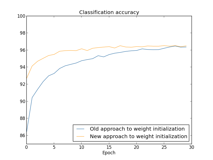
  In both cases, we end up with a classification accuracy somewhat over96 percent. The final classification accuracy is almost exactly thesame in the two cases. But the new initialization technique brings usthere much, much faster. At the end of the first epoch of trainingthe old approach to weight initialization has a classificationaccuracy under 87 percent, while the new approach is already almost 93percent. What appears to be going on is that our new approach toweight initialization starts us off in a much better regime, whichlets us get good results much more quickly. The same phenomenon isalso seen if we plot results with 100

  hidden neurons:

  

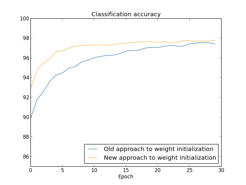
  In this case, the two curves don't quite meet. However, myexperiments suggest that with just a few more epochs of training (notshown) the accuracies become almost exactly the same. So on the basisof these experiments it looks as though the improved weightinitialization only speeds up learning, it doesn't change the finalperformance of our networks. However, in Chapter 4 we'll see examplesof neural networks where the long-run behaviour is significantlybetter with the 1/nin−−−√

  weight initialization. Thusit's not only the speed of learning which is improved, it's sometimesalso the final performance.

  The 1/nin−−−√

  approach to weight initialization helpsimprove the way our neural nets learn. Other techniques for weightinitialization have also been proposed, many building on this basicidea. I won't review the other approaches here, since 1/nin−−−√

  works well enough for our purposes. If you're interested inlooking further, I recommend looking at the discussion on pages 14 and15 of a 2012 paper by YoshuaBengio**Practical Recommendations for Gradient-Based Training of Deep Architectures, by Yoshua Bengio (2012)., as well as thereferences therein.

  Problem

  • Connecting regularization and the improved method of weight initialization L2 regularization sometimes automatically gives us something similar to the new approach to weight initialization. Suppose we are using the old approach to weight initialization. Sketch a heuristic argument that: (1) supposing λ
  is not too small, the first epochs of training will be dominated almost entirely by weight decay; (2) provided ηλ≪n the weights will decay by a factor of exp(−ηλ/m) per epoch; and (3) supposing λ is not too large, the weight decay will tail off when the weights are down to a size around 1/n√ , where n
  • is the total number of weights in the network. Argue that these conditions are all satisfied in the examples graphed in this section.

  Handwriting recognition revisited: the code

  Let's implement the ideas we've discussed in this chapter. We'lldevelop a new program,network2.py,which is an improved version of the programnetwork.pywe developed inChapter 1. If you haven't looked at network.py in a while then youmay find it helpful to spend a few minutes quickly reading over theearlier discussion. It's only 74 lines of code, and is easilyunderstood.

  As was the case in network.py, the star of network2.pyis the Network class, which we use to represent our neuralnetworks. We initialize an instance of Network with a list ofsizes for the respective layers in the network, and a choicefor the cost to use, defaulting to the cross-entropy:

  class Network(object):
  
      def __init__(self, sizes, cost=CrossEntropyCost):
          self.num_layers = len(sizes)
          self.sizes = sizes
          self.default_weight_initializer()
          self.cost=cost
  

  The first couple of lines of the __init__ method are the sameas in network.py, and are pretty self-explanatory. But thenext two lines are new, and we need to understand what they're doingin detail.

  Let's start by examining the default_weight_initializermethod. This makes use of our new and improved approach to weight initialization. As we've seen, in thatapproach the weights input to a neuron are initialized as Gaussianrandom variables with mean 0 and standard deviation 1

  divided by thesquare root of the number of connections input to the neuron. Also inthis method we'll initialize the biases, using Gaussian randomvariables with mean 0 and standard deviation 1

  . Here's the code:

      def default_weight_initializer(self):
          self.biases = [np.random.randn(y, 1) for y in self.sizes[1:]]
          self.weights = [np.random.randn(y, x)/np.sqrt(x) 
                          for x, y in zip(self.sizes[:-1], self.sizes[1:])]
  

  To understand the code, it may help to recall that np is theNumpy library for doing linear algebra. We'll import Numpy atthe beginning of our program. Also, notice that we don't initializeany biases for the first layer of neurons. We avoid doing thisbecause the first layer is an input layer, and so any biases would notbe used. We did exactly the same thing in network.py.

  Complementing the default_weight_initializer we'll also includea large_weight_initializer method. This method initializes theweights and biases using the old approach from Chapter 1, with bothweights and biases initialized as Gaussian random variables with mean 0

  and standard deviation 1

  . The code is, of course, only a tinybit different from the default_weight_initializer:

      def large_weight_initializer(self):
          self.biases = [np.random.randn(y, 1) for y in self.sizes[1:]]
          self.weights = [np.random.randn(y, x) 
                          for x, y in zip(self.sizes[:-1], self.sizes[1:])]
  

  I've included the large_weight_initializer method mostly as aconvenience to make it easier to compare the results in this chapterto those in Chapter 1. I can't think of many practical situationswhere I would recommend using it!

  The second new thing in Network's __init__ method isthat we now initialize a cost attribute. To understand howthat works, let's look at the class we use to represent thecross-entropy cost**If you're not familiar with Python's static methods you can ignore the @staticmethod decorators, and just treat fn and delta as ordinary methods. If you're curious about details, all @staticmethod does is tell the Python interpreter that the method which follows doesn't depend on the object in any way. That's why self isn't passed as a parameter to the fn and delta methods.:

  class CrossEntropyCost(object):
  
      @staticmethod
      def fn(a, y):
          return np.sum(np.nan_to_num(-y*np.log(a)-(1-y)*np.log(1-a)))
  
      @staticmethod
      def delta(z, a, y):
          return (a-y)
  

  Let's break this down. The first thing to observe is that even thoughthe cross-entropy is, mathematically speaking, a function, we'veimplemented it as a Python class, not a Python function. Why have Imade that choice? The reason is that the cost plays two differentroles in our network. The obvious role is that it's a measure of howwell an output activation, a, matches the desired output,y. This role is captured by the CrossEntropyCost.fnmethod. (Note, by the way, that the np.nan_to_num call insideCrossEntropyCost.fn ensures that Numpy deals correctly with thelog of numbers very close to zero.) But there's also a second way thecost function enters our network. Recall fromChapter 2 that when running the backpropagation algorithm we need tocompute the network's output error, δL

  . The form of the outputerror depends on the choice of cost function: different cost function,different form for the output error. For the cross-entropy the outputerror is, as we saw in Equation (66),

  δL=aL−y.(99)

  For this reason we define a second method,CrossEntropyCost.delta, whose purpose is to tell our networkhow to compute the output error. And then we bundle these two methodsup into a single class containing everything our networks need to knowabout the cost function.

  In a similar way, network2.py also contains a class torepresent the quadratic cost function. This is included forcomparison with the results of Chapter 1, since going forward we'llmostly use the cross entropy. The code is just below. TheQuadraticCost.fn method is a straightforward computation of thequadratic cost associated to the actual output, a, and thedesired output, y. The value returned byQuadraticCost.delta is based on theexpression (30) for the output error for thequadratic cost, which we derived back in Chapter 2.

  class QuadraticCost(object):
  
      @staticmethod
      def fn(a, y):
          return 0.5*np.linalg.norm(a-y)**2
  
      @staticmethod
      def delta(z, a, y):
          return (a-y) * sigmoid_prime(z)
  

  We've now understood the main differences between network2.pyand network.py. It's all pretty simple stuff. There are anumber of smaller changes, which I'll discuss below, including theimplementation of L2 regularization. Before getting to that, let'slook at the complete code for network2.py. You don't need toread all the code in detail, but it is worth understanding the broadstructure, and in particular reading the documentation strings, so youunderstand what each piece of the program is doing. Of course, you'realso welcome to delve as deeply as you wish! If you get lost, you maywish to continue reading the prose below, and return to the codelater. Anyway, here's the code:

  """network2.py
  ~~~~~~~~~~~~~~
  
  An improved version of network.py, implementing the stochastic
  gradient descent learning algorithm for a feedforward neural network.
  Improvements include the addition of the cross-entropy cost function,
  regularization, and better initialization of network weights.  Note
  that I have focused on making the code simple, easily readable, and
  easily modifiable.  It is not optimized, and omits many desirable
  features.
  
  """
  
  #### Libraries
  # Standard library
  import json
  import random
  import sys
  
  # Third-party libraries
  import numpy as np
  
  
  #### Define the quadratic and cross-entropy cost functions
  
  class QuadraticCost(object):
  
      @staticmethod
      def fn(a, y):
          """Return the cost associated with an output ``a`` and desired output
          ``y``.
  
          """
          return 0.5*np.linalg.norm(a-y)**2
  
      @staticmethod
      def delta(z, a, y):
          """Return the error delta from the output layer."""
          return (a-y) * sigmoid_prime(z)
  
  
  class CrossEntropyCost(object):
  
      @staticmethod
      def fn(a, y):
          """Return the cost associated with an output ``a`` and desired output
          ``y``.  Note that np.nan_to_num is used to ensure numerical
          stability.  In particular, if both ``a`` and ``y`` have a 1.0
          in the same slot, then the expression (1-y)*np.log(1-a)
          returns nan.  The np.nan_to_num ensures that that is converted
          to the correct value (0.0).
  
          """
          return np.sum(np.nan_to_num(-y*np.log(a)-(1-y)*np.log(1-a)))
  
      @staticmethod
      def delta(z, a, y):
          """Return the error delta from the output layer.  Note that the
          parameter ``z`` is not used by the method.  It is included in
          the method's parameters in order to make the interface
          consistent with the delta method for other cost classes.
  
          """
          return (a-y)
  
  
  #### Main Network class
  class Network(object):
  
      def __init__(self, sizes, cost=CrossEntropyCost):
          """The list ``sizes`` contains the number of neurons in the respective
          layers of the network.  For example, if the list was [2, 3, 1]
          then it would be a three-layer network, with the first layer
          containing 2 neurons, the second layer 3 neurons, and the
          third layer 1 neuron.  The biases and weights for the network
          are initialized randomly, using
          ``self.default_weight_initializer`` (see docstring for that
          method).
  
          """
          self.num_layers = len(sizes)
          self.sizes = sizes
          self.default_weight_initializer()
          self.cost=cost
  
      def default_weight_initializer(self):
          """Initialize each weight using a Gaussian distribution with mean 0
          and standard deviation 1 over the square root of the number of
          weights connecting to the same neuron.  Initialize the biases
          using a Gaussian distribution with mean 0 and standard
          deviation 1.
  
          Note that the first layer is assumed to be an input layer, and
          by convention we won't set any biases for those neurons, since
          biases are only ever used in computing the outputs from later
          layers.
  
          """
          self.biases = [np.random.randn(y, 1) for y in self.sizes[1:]]
          self.weights = [np.random.randn(y, x)/np.sqrt(x)
                          for x, y in zip(self.sizes[:-1], self.sizes[1:])]
  
      def large_weight_initializer(self):
          """Initialize the weights using a Gaussian distribution with mean 0
          and standard deviation 1.  Initialize the biases using a
          Gaussian distribution with mean 0 and standard deviation 1.
  
          Note that the first layer is assumed to be an input layer, and
          by convention we won't set any biases for those neurons, since
          biases are only ever used in computing the outputs from later
          layers.
  
          This weight and bias initializer uses the same approach as in
          Chapter 1, and is included for purposes of comparison.  It
          will usually be better to use the default weight initializer
          instead.
  
          """
          self.biases = [np.random.randn(y, 1) for y in self.sizes[1:]]
          self.weights = [np.random.randn(y, x)
                          for x, y in zip(self.sizes[:-1], self.sizes[1:])]
  
      def feedforward(self, a):
          """Return the output of the network if ``a`` is input."""
          for b, w in zip(self.biases, self.weights):
              a = sigmoid(np.dot(w, a)+b)
          return a
  
      def SGD(self, training_data, epochs, mini_batch_size, eta,
              lmbda = 0.0,
              evaluation_data=None,
              monitor_evaluation_cost=False,
              monitor_evaluation_accuracy=False,
              monitor_training_cost=False,
              monitor_training_accuracy=False):
          """Train the neural network using mini-batch stochastic gradient
          descent.  The ``training_data`` is a list of tuples ``(x, y)``
          representing the training inputs and the desired outputs.  The
          other non-optional parameters are self-explanatory, as is the
          regularization parameter ``lmbda``.  The method also accepts
          ``evaluation_data``, usually either the validation or test
          data.  We can monitor the cost and accuracy on either the
          evaluation data or the training data, by setting the
          appropriate flags.  The method returns a tuple containing four
          lists: the (per-epoch) costs on the evaluation data, the
          accuracies on the evaluation data, the costs on the training
          data, and the accuracies on the training data.  All values are
          evaluated at the end of each training epoch.  So, for example,
          if we train for 30 epochs, then the first element of the tuple
          will be a 30-element list containing the cost on the
          evaluation data at the end of each epoch. Note that the lists
          are empty if the corresponding flag is not set.
  
          """
          if evaluation_data: n_data = len(evaluation_data)
          n = len(training_data)
          evaluation_cost, evaluation_accuracy = [], []
          training_cost, training_accuracy = [], []
          for j in xrange(epochs):
              random.shuffle(training_data)
              mini_batches = [
                  training_data[k:k+mini_batch_size]
                  for k in xrange(0, n, mini_batch_size)]
              for mini_batch in mini_batches:
                  self.update_mini_batch(
                      mini_batch, eta, lmbda, len(training_data))
              print "Epoch %s training complete" % j
              if monitor_training_cost:
                  cost = self.total_cost(training_data, lmbda)
                  training_cost.append(cost)
                  print "Cost on training data: {}".format(cost)
              if monitor_training_accuracy:
                  accuracy = self.accuracy(training_data, convert=True)
                  training_accuracy.append(accuracy)
                  print "Accuracy on training data: {} / {}".format(
                      accuracy, n)
              if monitor_evaluation_cost:
                  cost = self.total_cost(evaluation_data, lmbda, convert=True)
                  evaluation_cost.append(cost)
                  print "Cost on evaluation data: {}".format(cost)
              if monitor_evaluation_accuracy:
                  accuracy = self.accuracy(evaluation_data)
                  evaluation_accuracy.append(accuracy)
                  print "Accuracy on evaluation data: {} / {}".format(
                      self.accuracy(evaluation_data), n_data)
              print
          return evaluation_cost, evaluation_accuracy, \
              training_cost, training_accuracy
  
      def update_mini_batch(self, mini_batch, eta, lmbda, n):
          """Update the network's weights and biases by applying gradient
          descent using backpropagation to a single mini batch.  The
          ``mini_batch`` is a list of tuples ``(x, y)``, ``eta`` is the
          learning rate, ``lmbda`` is the regularization parameter, and
          ``n`` is the total size of the training data set.
  
          """
          nabla_b = [np.zeros(b.shape) for b in self.biases]
          nabla_w = [np.zeros(w.shape) for w in self.weights]
          for x, y in mini_batch:
              delta_nabla_b, delta_nabla_w = self.backprop(x, y)
              nabla_b = [nb+dnb for nb, dnb in zip(nabla_b, delta_nabla_b)]
              nabla_w = [nw+dnw for nw, dnw in zip(nabla_w, delta_nabla_w)]
          self.weights = [(1-eta*(lmbda/n))*w-(eta/len(mini_batch))*nw
                          for w, nw in zip(self.weights, nabla_w)]
          self.biases = [b-(eta/len(mini_batch))*nb
                         for b, nb in zip(self.biases, nabla_b)]
  
      def backprop(self, x, y):
          """Return a tuple ``(nabla_b, nabla_w)`` representing the
          gradient for the cost function C_x.  ``nabla_b`` and
          ``nabla_w`` are layer-by-layer lists of numpy arrays, similar
          to ``self.biases`` and ``self.weights``."""
          nabla_b = [np.zeros(b.shape) for b in self.biases]
          nabla_w = [np.zeros(w.shape) for w in self.weights]
          # feedforward
          activation = x
          activations = [x] # list to store all the activations, layer by layer
          zs = [] # list to store all the z vectors, layer by layer
          for b, w in zip(self.biases, self.weights):
              z = np.dot(w, activation)+b
              zs.append(z)
              activation = sigmoid(z)
              activations.append(activation)
          # backward pass
          delta = (self.cost).delta(zs[-1], activations[-1], y)
          nabla_b[-1] = delta
          nabla_w[-1] = np.dot(delta, activations[-2].transpose())
          # Note that the variable l in the loop below is used a little
          # differently to the notation in Chapter 2 of the book.  Here,
          # l = 1 means the last layer of neurons, l = 2 is the
          # second-last layer, and so on.  It's a renumbering of the
          # scheme in the book, used here to take advantage of the fact
          # that Python can use negative indices in lists.
          for l in xrange(2, self.num_layers):
              z = zs[-l]
              sp = sigmoid_prime(z)
              delta = np.dot(self.weights[-l+1].transpose(), delta) * sp
              nabla_b[-l] = delta
              nabla_w[-l] = np.dot(delta, activations[-l-1].transpose())
          return (nabla_b, nabla_w)
  
      def accuracy(self, data, convert=False):
          """Return the number of inputs in ``data`` for which the neural
          network outputs the correct result. The neural network's
          output is assumed to be the index of whichever neuron in the
          final layer has the highest activation.
  
          The flag ``convert`` should be set to False if the data set is
          validation or test data (the usual case), and to True if the
          data set is the training data. The need for this flag arises
          due to differences in the way the results ``y`` are
          represented in the different data sets.  In particular, it
          flags whether we need to convert between the different
          representations.  It may seem strange to use different
          representations for the different data sets.  Why not use the
          same representation for all three data sets?  It's done for
          efficiency reasons -- the program usually evaluates the cost
          on the training data and the accuracy on other data sets.
          These are different types of computations, and using different
          representations speeds things up.  More details on the
          representations can be found in
          mnist_loader.load_data_wrapper.
  
          """
          if convert:
              results = [(np.argmax(self.feedforward(x)), np.argmax(y))
                         for (x, y) in data]
          else:
              results = [(np.argmax(self.feedforward(x)), y)
                          for (x, y) in data]
          return sum(int(x == y) for (x, y) in results)
  
      def total_cost(self, data, lmbda, convert=False):
          """Return the total cost for the data set ``data``.  The flag
          ``convert`` should be set to False if the data set is the
          training data (the usual case), and to True if the data set is
          the validation or test data.  See comments on the similar (but
          reversed) convention for the ``accuracy`` method, above.
          """
          cost = 0.0
          for x, y in data:
              a = self.feedforward(x)
              if convert: y = vectorized_result(y)
              cost += self.cost.fn(a, y)/len(data)
          cost += 0.5*(lmbda/len(data))*sum(
              np.linalg.norm(w)**2 for w in self.weights)
          return cost
  
      def save(self, filename):
          """Save the neural network to the file ``filename``."""
          data = {"sizes": self.sizes,
                  "weights": [w.tolist() for w in self.weights],
                  "biases": [b.tolist() for b in self.biases],
                  "cost": str(self.cost.__name__)}
          f = open(filename, "w")
          json.dump(data, f)
          f.close()
  
  #### Loading a Network
  def load(filename):
      """Load a neural network from the file ``filename``.  Returns an
      instance of Network.
  
      """
      f = open(filename, "r")
      data = json.load(f)
      f.close()
      cost = getattr(sys.modules[__name__], data["cost"])
      net = Network(data["sizes"], cost=cost)
      net.weights = [np.array(w) for w in data["weights"]]
      net.biases = [np.array(b) for b in data["biases"]]
      return net
  
  #### Miscellaneous functions
  def vectorized_result(j):
      """Return a 10-dimensional unit vector with a 1.0 in the j'th position
      and zeroes elsewhere.  This is used to convert a digit (0...9)
      into a corresponding desired output from the neural network.
  
      """
      e = np.zeros((10, 1))
      e[j] = 1.0
      return e
  
  def sigmoid(z):
      """The sigmoid function."""
      return 1.0/(1.0+np.exp(-z))
  
  def sigmoid_prime(z):
      """Derivative of the sigmoid function."""
      return sigmoid(z)*(1-sigmoid(z))
  

  One of the more interesting changes in the code is to include L2regularization. Although this is a major conceptual change, it's sotrivial to implement that it's easy to miss in the code. For the mostpart it just involves passing the parameter lmbda to variousmethods, notably the Network.SGD method. The real work is donein a single line of the program, the fourth-last line of theNetwork.update_mini_batch method. That's where we modify thegradient descent update rule to include weight decay. But althoughthe modification is tiny, it has a big impact on results!

  This is, by the way, common when implementing new techniques in neuralnetworks. We've spent thousands of words discussing regularization.It's conceptually quite subtle and difficult to understand. And yetit was trivial to add to our program! It occurs surprisingly oftenthat sophisticated techniques can be implemented with small changes tocode.

  Another small but important change to our code is the addition ofseveral optional flags to the stochastic gradient descent method,Network.SGD. These flags make it possible to monitor the costand accuracy either on the training_data or on a set ofevaluation_data which can be passed to Network.SGD.We've used these flags often earlier in the chapter, but let me givean example of how it works, just to remind you:

  >>> import mnist_loader
  >>> training_data, validation_data, test_data = \
  ... mnist_loader.load_data_wrapper()
  >>> import network2
  >>> net = network2.Network([784, 30, 10], cost=network2.CrossEntropyCost)
  >>> net.SGD(training_data, 30, 10, 0.5,
  ... lmbda = 5.0,
  ... evaluation_data=validation_data,
  ... monitor_evaluation_accuracy=True,
  ... monitor_evaluation_cost=True,
  ... monitor_training_accuracy=True,
  ... monitor_training_cost=True)
  

  Here, we're setting the evaluation_data to be thevalidation_data. But we could also have monitored performanceon the test_data or any other data set. We also have fourflags telling us to monitor the cost and accuracy on both theevaluation_data and the training_data. Those flags areFalse by default, but they've been turned on here in order tomonitor our Network's performance. Furthermore,network2.py's Network.SGD method returns a four-elementtuple representing the results of the monitoring. We can use this asfollows:

  >>> evaluation_cost, evaluation_accuracy, 
  ... training_cost, training_accuracy = net.SGD(training_data, 30, 10, 0.5,
  ... lmbda = 5.0,
  ... evaluation_data=validation_data,
  ... monitor_evaluation_accuracy=True,
  ... monitor_evaluation_cost=True,
  ... monitor_training_accuracy=True,
  ... monitor_training_cost=True)
  

  So, for example, evaluation_cost will be a 30-element listcontaining the cost on the evaluation data at the end of each epoch.This sort of information is extremely useful in understanding anetwork's behaviour. It can, for example, be used to draw graphsshowing how the network learns over time. Indeed, that's exactly howI constructed all the graphs earlier in the chapter. Note, however,that if any of the monitoring flags are not set, then thecorresponding element in the tuple will be the empty list.

  Other additions to the code include a Network.save method, tosave Network objects to disk, and a function to loadthem back in again later. Note that the saving and loading is doneusing JSON, not Python's pickle or cPickle modules,which are the usual way we save and load objects to and from disk inPython. Using JSON requires more code than pickle orcPickle would. To understand why I've used JSON, imagine thatat some time in the future we decided to change our Networkclass to allow neurons other than sigmoid neurons. To implement thatchange we'd most likely change the attributes defined in theNetwork.__init__ method. If we've simply pickled the objectsthat would cause our load function to fail. Using JSON to dothe serialization explicitly makes it easy to ensure that oldNetworks will still load.

  There are many other minor changes in the code for network2.py,but they're all simple variations on network.py. The netresult is to expand our 74-line program to a far more capable 152lines.

  Problems

  • Modify the code above to implement L1 regularization, and use L1 regularization to classify MNIST digits using a 30
  • hidden neuron network. Can you find a regularization parameter that enables you to do better than running unregularized?
  • Take a look at the Network.cost_derivative method in network.py. That method was written for the quadratic cost. How would you rewrite the method for the cross-entropy cost? Can you think of a problem that might arise in the cross-entropy version? In network2.py we've eliminated the Network.cost_derivative method entirely, instead incorporating its functionality into the CrossEntropyCost.delta method. How does this solve the problem you've just identified?

  How to choose a neural network's hyper-parameters?

  Up until now I haven't explained how I've been choosing values forhyper-parameters such as the learning rate, η

  , the regularizationparameter, λ , and so on. I've just been supplying valueswhich work pretty well. In practice, when you're using neural nets toattack a problem, it can be difficult to find good hyper-parameters.Imagine, for example, that we've just been introduced to the MNISTproblem, and have begun working on it, knowing nothing at all aboutwhat hyper-parameters to use. Let's suppose that by good fortune inour first experiments we choose many of the hyper-parameters in thesame way as was done earlier this chapter: 30 hidden neurons, amini-batch size of 10, training for 30 epochs using the cross-entropy.But we choose a learning rate η=10.0 and regularizationparameter λ=1000.0

  . Here's what I saw on one such run:

  >>> import mnist_loader
  >>> training_data, validation_data, test_data = \
  ... mnist_loader.load_data_wrapper()
  >>> import network2
  >>> net = network2.Network([784, 30, 10])
  >>> net.SGD(training_data, 30, 10, 10.0, lmbda = 1000.0,
  ... evaluation_data=validation_data, monitor_evaluation_accuracy=True)
  Epoch 0 training complete
  Accuracy on evaluation data: 1030 / 10000
  
  Epoch 1 training complete
  Accuracy on evaluation data: 990 / 10000
  
  Epoch 2 training complete
  Accuracy on evaluation data: 1009 / 10000
  
  ...
  
  Epoch 27 training complete
  Accuracy on evaluation data: 1009 / 10000
  
  Epoch 28 training complete
  Accuracy on evaluation data: 983 / 10000
  
  Epoch 29 training complete
  Accuracy on evaluation data: 967 / 10000
  

  Our classification accuracies are no better than chance! Our networkis acting as a random noise generator!

  "Well, that's easy to fix," you might say, "just decrease thelearning rate and regularization hyper-parameters". Unfortunately,you don't a priori know those are the hyper-parameters you needto adjust. Maybe the real problem is that our 30 hidden neuronnetwork will never work well, no matter how the other hyper-parametersare chosen? Maybe we really need at least 100 hidden neurons? Or 300hidden neurons? Or multiple hidden layers? Or a different approachto encoding the output? Maybe our network is learning, but we need totrain for more epochs? Maybe the mini-batches are too small? Maybewe'd do better switching back to the quadratic cost function? Maybewe need to try a different approach to weight initialization? And soon, on and on and on. It's easy to feel lost in hyper-parameterspace. This can be particularly frustrating if your network is verylarge, or uses a lot of training data, since you may train for hoursor days or weeks, only to get no result. If the situation persists,it damages your confidence. Maybe neural networks are the wrongapproach to your problem? Maybe you should quit your job and take upbeekeeping?

  In this section I explain some heuristics which can be used to set thehyper-parameters in a neural network. The goal is to help you developa workflow that enables you to do a pretty good job settinghyper-parameters. Of course, I won't cover everything abouthyper-parameter optimization. That's a huge subject, and it's not, inany case, a problem that is ever completely solved, nor is thereuniversal agreement amongst practitioners on the right strategies touse. There's always one more trick you can try to eke out a bit moreperformance from your network. But the heuristics in this sectionshould get you started.

  Broad strategy: When using neural networks to attack a newproblem the first challenge is to get any non-trivial learning,i.e., for the network to achieve results better than chance. This canbe surprisingly difficult, especially when confronting a new class ofproblem. Let's look at some strategies you can use if you're havingthis kind of trouble.

  Suppose, for example, that you're attacking MNIST for the first time.You start out enthusiastic, but are a little discouraged when yourfirst network fails completely, as in the example above. The way togo is to strip the problem down. Get rid of all the training andvalidation images except images which are 0s or 1s. Then try to traina network to distinguish 0s from 1s. Not only is that an inherentlyeasier problem than distinguishing all ten digits, it also reduces theamount of training data by 80 percent, speeding up training by afactor of 5. That enables much more rapid experimentation, and sogives you more rapid insight into how to build a good network.

  You can further speed up experimentation by stripping your networkdown to the simplest network likely to do meaningful learning. If youbelieve a [784, 10] network can likely do better-than-chanceclassification of MNIST digits, then begin your experimentation withsuch a network. It'll be much faster than training a[784, 30, 10] network, and you can build back up to the latter.

  You can get another speed up in experimentation by increasing thefrequency of monitoring. In network2.py we monitor performanceat the end of each training epoch. With 50,000 images per epoch, thatmeans waiting a little while - about ten seconds per epoch, on mylaptop, when training a [784, 30, 10] network - beforegetting feedback on how well the network is learning. Of course, tenseconds isn't very long, but if you want to trial dozens ofhyper-parameter choices it's annoying, and if you want to trialhundreds or thousands of choices it starts to get debilitating. Wecan get feedback more quickly by monitoring the validation accuracymore often, say, after every 1,000 training images. Furthermore,instead of using the full 10,000 image validation set to monitorperformance, we can get a much faster estimate using just 100validation images. All that matters is that the network sees enoughimages to do real learning, and to get a pretty good rough estimate ofperformance. Of course, our program network2.py doesn'tcurrently do this kind of monitoring. But as a kludge to achieve asimilar effect for the purposes of illustration, we'll strip down ourtraining data to just the first 1,000 MNIST training images. Let'stry it and see what happens. (To keep the code below simple I haven'timplemented the idea of using only 0 and 1 images. Of course, thatcan be done with just a little more work.)

  >>> net = network2.Network([784, 10])
  >>> net.SGD(training_data[:1000], 30, 10, 10.0, lmbda = 1000.0, \
  ... evaluation_data=validation_data[:100], \
  ... monitor_evaluation_accuracy=True)
  Epoch 0 training complete
  Accuracy on evaluation data: 10 / 100
  
  Epoch 1 training complete
  Accuracy on evaluation data: 10 / 100
  
  Epoch 2 training complete
  Accuracy on evaluation data: 10 / 100
  ...
  

  We're still getting pure noise! But there's a big win: we're nowgetting feedback in a fraction of a second, rather than once every tenseconds or so. That means you can more quickly experiment with otherchoices of hyper-parameter, or even conduct experiments trialling manydifferent choices of hyper-parameter nearly simultaneously.

  In the above example I left λ

  as λ=1000.0 , as weused earlier. But since we changed the number of training examples weshould really change λ to keep the weight decay the same.That means changing λ to 20.0

  . If we do that then this iswhat happens:

  >>> net = network2.Network([784, 10])
  >>> net.SGD(training_data[:1000], 30, 10, 10.0, lmbda = 20.0, \
  ... evaluation_data=validation_data[:100], \
  ... monitor_evaluation_accuracy=True)
  Epoch 0 training complete
  Accuracy on evaluation data: 12 / 100
  
  Epoch 1 training complete
  Accuracy on evaluation data: 14 / 100
  
  Epoch 2 training complete
  Accuracy on evaluation data: 25 / 100
  
  Epoch 3 training complete
  Accuracy on evaluation data: 18 / 100
  ...
  

  Ahah! We have a signal. Not a terribly good signal, but a signalnonetheless. That's something we can build on, modifying thehyper-parameters to try to get further improvement. Maybe we guessthat our learning rate needs to be higher. (As you perhaps realize,that's a silly guess, for reasons we'll discuss shortly, but pleasebear with me.) So to test our guess we try dialing η

  up to 100.0

  :

  >>> net = network2.Network([784, 10])
  >>> net.SGD(training_data[:1000], 30, 10, 100.0, lmbda = 20.0, \
  ... evaluation_data=validation_data[:100], \
  ... monitor_evaluation_accuracy=True)
  Epoch 0 training complete
  Accuracy on evaluation data: 10 / 100
  
  Epoch 1 training complete
  Accuracy on evaluation data: 10 / 100
  
  Epoch 2 training complete
  Accuracy on evaluation data: 10 / 100
  
  Epoch 3 training complete
  Accuracy on evaluation data: 10 / 100
  
  ...
  

  That's no good! It suggests that our guess was wrong, and the problemwasn't that the learning rate was too low. So instead we try dialing η

  down to η=1.0

  :

  >>> net = network2.Network([784, 10])
  >>> net.SGD(training_data[:1000], 30, 10, 1.0, lmbda = 20.0, \
  ... evaluation_data=validation_data[:100], \
  ... monitor_evaluation_accuracy=True)
  Epoch 0 training complete
  Accuracy on evaluation data: 62 / 100
  
  Epoch 1 training complete
  Accuracy on evaluation data: 42 / 100
  
  Epoch 2 training complete
  Accuracy on evaluation data: 43 / 100
  
  Epoch 3 training complete
  Accuracy on evaluation data: 61 / 100
  
  ...
  

  That's better! And so we can continue, individually adjusting eachhyper-parameter, gradually improving performance. Once we've exploredto find an improved value for η

  , then we move on to find a goodvalue for λ . Then experiment with a more complexarchitecture, say a network with 10 hidden neurons. Then adjust thevalues for η and λ

  again. Then increase to 20 hiddenneurons. And then adjust other hyper-parameters some more. And soon, at each stage evaluating performance using our held-out validationdata, and using those evaluations to find better and betterhyper-parameters. As we do so, it typically takes longer to witnessthe impact due to modifications of the hyper-parameters, and so we cangradually decrease the frequency of monitoring.

  This all looks very promising as a broad strategy. However, I want toreturn to that initial stage of finding hyper-parameters that enable anetwork to learn anything at all. In fact, even the above discussionconveys too positive an outlook. It can be immensely frustrating towork with a network that's learning nothing. You can tweakhyper-parameters for days, and still get no meaningful response. Andso I'd like to re-emphasize that during the early stages you shouldmake sure you can get quick feedback from experiments. Intuitively,it may seem as though simplifying the problem and the architecturewill merely slow you down. In fact, it speeds things up, since youmuch more quickly find a network with a meaningful signal. Onceyou've got such a signal, you can often get rapid improvements bytweaking the hyper-parameters. As with many things in life, gettingstarted can be the hardest thing to do.

  Okay, that's the broad strategy. Let's now look at some specificrecommendations for setting hyper-parameters. I will focus on thelearning rate, η

  , the L2 regularization parameter, λ

  , andthe mini-batch size. However, many of the remarks apply also to otherhyper-parameters, including those associated to network architecture,other forms of regularization, and some hyper-parameters we'll meetlater in the book, such as the momentum co-efficient.

  Learning rate: Suppose we run three MNIST networks with threedifferent learning rates, η=0.025

  , η=0.25 and η=2.5 , respectively. We'll set the other hyper-parameters as for theexperiments in earlier sections, running over 30 epochs, with amini-batch size of 10, and with λ=5.0 . We'll also return tousing the full 50,000

  training images. Here's a graph showing thebehaviour of the training cost as we train**The graph was generated by multiple_eta.py.:

  

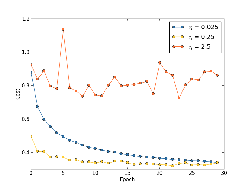
  With η=0.025

  the cost decreases smoothly until the final epoch.With η=0.25 the cost initially decreases, but after about 20 epochs it is near saturation, and thereafter most of the changes aremerely small and apparently random oscillations. Finally, with η=2.5

  the cost makes large oscillations right from the start. Tounderstand the reason for the oscillations, recall that stochasticgradient descent is supposed to step us gradually down into a valleyof the cost function,

  

  However, if η

  is too large then the steps will be so large thatthey may actually overshoot the minimum, causing the algorithm toclimb up out of the valley instead. That's likely**This picture is helpful, but it's intended as an intuition-building illustration of what may go on, not as a complete, exhaustive explanation. Briefly, a more complete explanation is as follows: gradient descent uses a first-order approximation to the cost function as a guide to how to decrease the cost. For large η , higher-order terms in the cost function become more important, and may dominate the behaviour, causing gradient descent to break down. This is especially likely as we approach minima and quasi-minima of the cost function, since near such points the gradient becomes small, making it easier for higher-order terms to dominate behaviour. what's causing the cost to oscillate when η=2.5 .When we choose η=0.25 the initial steps do take us toward aminimum of the cost function, and it's only once we get near thatminimum that we start to suffer from the overshooting problem. Andwhen we choose η=0.025 we don't suffer from this problem at allduring the first 30 epochs. Of course, choosing η so smallcreates another problem, namely, that it slows down stochasticgradient descent. An even better approach would be to start with η=0.25 , train for 20 epochs, and then switch to η=0.025 . We'll discuss such variable learning rate schedules later.For now, though, let's stick to figuring out how to find a single goodvalue for the learning rate, η

  .

  With this picture in mind, we can set η

  as follows. First, weestimate the threshold value for η at which the cost on thetraining data immediately begins decreasing, instead of oscillating orincreasing. This estimate doesn't need to be too accurate. You canestimate the order of magnitude by starting with η=0.01 . Ifthe cost decreases during the first few epochs, then you shouldsuccessively try η=0.1,1.0,… until you find a value for η where the cost oscillates or increases during the first fewepochs. Alternately, if the cost oscillates or increases during thefirst few epochs when η=0.01 , then try η=0.001,0.0001,… until you find a value for η where the cost decreasesduring the first few epochs. Following this procedure will give us anorder of magnitude estimate for the threshold value of η . Youmay optionally refine your estimate, to pick out the largest value of η at which the cost decreases during the first few epochs, say η=0.5 or η=0.2 (there's no need for this to besuper-accurate). This gives us an estimate for the threshold value of η

  .

  Obviously, the actual value of η

  that you use should be no largerthan the threshold value. In fact, if the value of η is toremain usable over many epochs then you likely want to use a valuefor η

  that is smaller, say, a factor of two below the threshold.Such a choice will typically allow you to train for many epochs,without causing too much of a slowdown in learning.

  In the case of the MNIST data, following this strategy leads to anestimate of 0.1

  for the order of magnitude of the threshold value of η . After some more refinement, we obtain a threshold value η=0.5 . Following the prescription above, this suggests using η=0.25 as our value for the learning rate. In fact, I found that using η=0.5 worked well enough over 30 epochs that for the mostpart I didn't worry about using a lower value of η

  .

  This all seems quite straightforward. However, using the trainingcost to pick η

  appears to contradict what I said earlier in thissection, namely, that we'd pick hyper-parameters by evaluatingperformance using our held-out validation data. In fact, we'll usevalidation accuracy to pick the regularization hyper-parameter, themini-batch size, and network parameters such as the number of layersand hidden neurons, and so on. Why do things differently for thelearning rate? Frankly, this choice is my personal aestheticpreference, and is perhaps somewhat idiosyncratic. The reasoning isthat the other hyper-parameters are intended to improve the finalclassification accuracy on the test set, and so it makes sense toselect them on the basis of validation accuracy. However, thelearning rate is only incidentally meant to impact the finalclassification accuracy. Its primary purpose is really to controlthe step size in gradient descent, and monitoring the training cost isthe best way to detect if the step size is too big. With that said,this is a personal aesthetic preference. Early on during learning thetraining cost usually only decreases if the validation accuracyimproves, and so in practice it's unlikely to make much differencewhich criterion you use.

  Use early stopping to determine the number of training epochs: As we discussed earlier in the chapter, early stopping meansthat at the end of each epoch we should compute the classificationaccuracy on the validation data. When that stops improving,terminate. This makes setting the number of epochs very simple. Inparticular, it means that we don't need to worry about explicitlyfiguring out how the number of epochs depends on the otherhyper-parameters. Instead, that's taken care of automatically.Furthermore, early stopping also automatically prevents us fromoverfitting. This is, of course, a good thing, although in the earlystages of experimentation it can be helpful to turn off earlystopping, so you can see any signs of overfitting, and use it toinform your approach to regularization.

  To implement early stopping we need to say more precisely what itmeans that the classification accuracy has stopped improving. Aswe've seen, the accuracy can jump around quite a bit, even when theoverall trend is to improve. If we stop the first time the accuracydecreases then we'll almost certainly stop when there are moreimprovements to be had. A better rule is to terminate if the bestclassification accuracy doesn't improve for quite some time. Suppose,for example, that we're doing MNIST. Then we might elect to terminateif the classification accuracy hasn't improved during the last tenepochs. This ensures that we don't stop too soon, in response to badluck in training, but also that we're not waiting around forever foran improvement that never comes.

  This no-improvement-in-ten rule is good for initial exploration ofMNIST. However, networks can sometimes plateau near a particularclassification accuracy for quite some time, only to then beginimproving again. If you're trying to get really good performance, theno-improvement-in-ten rule may be too aggressive about stopping. Inthat case, I suggest using the no-improvement-in-ten rule for initialexperimentation, and gradually adopting more lenient rules, as youbetter understand the way your network trains:no-improvement-in-twenty, no-improvement-in-fifty, and so on. Ofcourse, this introduces a new hyper-parameter to optimize! Inpractice, however, it's usually easy to set this hyper-parameter toget pretty good results. Similarly, for problems other than MNIST,the no-improvement-in-ten rule may be much too aggressive or notnearly aggressive enough, depending on the details of the problem.However, with a little experimentation it's usually easy to find apretty good strategy for early stopping.

  We haven't used early stopping in our MNIST experiments to date. Thereason is that we've been doing a lot of comparisons between differentapproaches to learning. For such comparisons it's helpful to use thesame number of epochs in each case. However, it's well worthmodifying network2.py to implement early stopping:

  Problem

  • Modify network2.py so that it implements early stopping using a no-improvement-in- n
  epochs strategy, where n
• is a parameter that can be set.
• Can you think of a rule for early stopping other than no-improvement-in- n ? Ideally, the rule should compromise between getting high validation accuracies and not training too long. Add your rule to network2.py, and run three experiments comparing the validation accuracies and number of epochs of training to no-improvement-in- 10
  • .

  Learning rate schedule: We've been holding the learning rate η

  constant. However, it's often advantageous to vary thelearning rate. Early on during the learning process it's likely thatthe weights are badly wrong. And so it's best to use a large learningrate that causes the weights to change quickly. Later, we can reducethe learning rate as we make more fine-tuned adjustments to ourweights.

  How should we set our learning rate schedule? Many approaches arepossible. One natural approach is to use the same basic idea as earlystopping. The idea is to hold the learning rate constant until thevalidation accuracy starts to get worse. Then decrease the learningrate by some amount, say a factor of two or ten. We repeat this manytimes, until, say, the learning rate is a factor of 1,024 (or 1,000)times lower than the initial value. Then we terminate.

  A variable learning schedule can improve performance, but it alsoopens up a world of possible choices for the learning schedule. Thosechoices can be a headache - you can spend forever trying to optimizeyour learning schedule. For first experiments my suggestion is to usea single, constant value for the learning rate. That'll get you agood first approximation. Later, if you want to obtain the bestperformance from your network, it's worth experimenting with alearning schedule, along the lines I've described**A readable recent paper which demonstrates the benefits of variable learning rates in attacking MNIST is Deep, Big, Simple Neural Nets Excel on Handwritten Digit Recognition, by Dan Claudiu Cireșan, Ueli Meier, Luca Maria Gambardella, and Jürgen Schmidhuber (2010)..

  Exercise

  • Modify network2.py so that it implements a learning schedule that: halves the learning rate each time the validation accuracy satisfies the no-improvement-in- 10
  rule; and terminates when the learning rate has dropped to 1/128
  • of its original value.

  The regularization parameter, λ

  : I suggest startinginitially with no regularization ( λ=0.0 ), and determining avalue for η , as above. Using that choice of η , we can thenuse the validation data to select a good value for λ . Startby trialling λ=1.0 **I don't have a good principled justification for using this as a starting value. If anyone knows of a good principled discussion of where to start with λ , I'd appreciate hearing it (mn@michaelnielsen.org)., and thenincrease or decrease by factors of 10 , as needed to improveperformance on the validation data. Once you've found a good order ofmagnitude, you can fine tune your value of λ . That done, youshould return and re-optimize η

  again.

  Exercise

  • It's tempting to use gradient descent to try to learn good values for hyper-parameters such as λ
  and η . Can you think of an obstacle to using gradient descent to determine λ ? Can you think of an obstacle to using gradient descent to determine η
  • ?

  How I selected hyper-parameters earlier in this book: If youuse the recommendations in this section you'll find that you getvalues for η

  and λ

  which don't always exactly match thevalues I've used earlier in the book. The reason is that the book hasnarrative constraints that have sometimes made it impractical tooptimize the hyper-parameters. Think of all the comparisons we'vemade of different approaches to learning, e.g., comparing thequadratic and cross-entropy cost functions, comparing the old and newmethods of weight initialization, running with and withoutregularization, and so on. To make such comparisons meaningful, I'veusually tried to keep hyper-parameters constant across the approachesbeing compared (or to scale them in an appropriate way). Of course,there's no reason for the same hyper-parameters to be optimal for allthe different approaches to learning, so the hyper-parameters I'veused are something of a compromise.

  As an alternative to this compromise, I could have tried to optimizethe heck out of the hyper-parameters for every single approach tolearning. In principle that'd be a better, fairer approach, sincethen we'd see the best from every approach to learning. However,we've made dozens of comparisons along these lines, and in practice Ifound it too computationally expensive. That's why I've adopted thecompromise of using pretty good (but not necessarily optimal) choicesfor the hyper-parameters.

  Mini-batch size: How should we set the mini-batch size? Toanswer this question, let's first suppose that we're doing onlinelearning, i.e., that we're using a mini-batch size of 1

  .

  The obvious worry about online learning is that using mini-batcheswhich contain just a single training example will cause significanterrors in our estimate of the gradient. In fact, though, the errorsturn out to not be such a problem. The reason is that the individualgradient estimates don't need to be super-accurate. All we need is anestimate accurate enough that our cost function tends to keepdecreasing. It's as though you are trying to get to the NorthMagnetic Pole, but have a wonky compass that's 10-20 degrees off eachtime you look at it. Provided you stop to check the compassfrequently, and the compass gets the direction right on average,you'll end up at the North Magnetic Pole just fine.

  Based on this argument, it sounds as though we should use onlinelearning. In fact, the situation turns out to be more complicatedthan that. In a problem in the last chapter I pointed out that it's possible to use matrixtechniques to compute the gradient update for all examples in amini-batch simultaneously, rather than looping over them. Dependingon the details of your hardware and linear algebra library this canmake it quite a bit faster to compute the gradient estimate for amini-batch of (for example) size 100

  , rather than computing themini-batch gradient estimate by looping over the 100 trainingexamples separately. It might take (say) only 50 times as long,rather than 100

  times as long.

  Now, at first it seems as though this doesn't help us that much. Withour mini-batch of size 100

  the learning rule for the weights lookslike:
  w→w′=w−η1100∑x∇Cx,(100)
  where the sum is over training examples in the mini-batch. This isversus
  w→w′=w−η∇Cx(101)
  for online learning. Even if it only takes 50 times as long to dothe mini-batch update, it still seems likely to be better to do onlinelearning, because we'd be updating so much more frequently. Suppose,however, that in the mini-batch case we increase the learning rate bya factor 100 , so the update rule becomes
  w→w′=w−η∑x∇Cx.(102)
  That's a lot like doing 100 separate instances of online learningwith a learning rate of η . But it only takes 50 times as longas doing a single instance of online learning. Of course, it's nottruly the same as 100 instances of online learning, since in themini-batch the ∇Cx

  's are all evaluated for the same set ofweights, as opposed to the cumulative learning that occurs in theonline case. Still, it seems distinctly possible that using thelarger mini-batch would speed things up.

  With these factors in mind, choosing the best mini-batch size is acompromise. Too small, and you don't get to take full advantage ofthe benefits of good matrix libraries optimized for fast hardware.Too large and you're simply not updating your weights often enough.What you need is to choose a compromise value which maximizes thespeed of learning. Fortunately, the choice of mini-batch size atwhich the speed is maximized is relatively independent of the otherhyper-parameters (apart from the overall architecture), so you don'tneed to have optimized those hyper-parameters in order to find a goodmini-batch size. The way to go is therefore to use some acceptable(but not necessarily optimal) values for the other hyper-parameters,and then trial a number of different mini-batch sizes, scaling η

  as above. Plot the validation accuracy versus time (as in,real elapsed time, not epoch!), and choose whichever mini-batch sizegives you the most rapid improvement in performance. With themini-batch size chosen you can then proceed to optimize the otherhyper-parameters.

  Of course, as you've no doubt realized, I haven't done thisoptimization in our work. Indeed, our implementation doesn't use thefaster approach to mini-batch updates at all. I've simply used amini-batch size of 10

  without comment or explanation in nearly allexamples. Because of this, we could have sped up learning by reducingthe mini-batch size. I haven't done this, in part because I wanted toillustrate the use of mini-batches beyond size 1

  , and in partbecause my preliminary experiments suggested the speedup would berather modest. In practical implementations, however, we would mostcertainly implement the faster approach to mini-batch updates, andthen make an effort to optimize the mini-batch size, in order tomaximize our overall speed.

  Automated techniques: I've been describing these heuristicsas though you're optimizing your hyper-parameters by hand.Hand-optimization is a good way to build up a feel for how neuralnetworks behave. However, and unsurprisingly, a great deal of workhas been done on automating the process. A common technique isgrid search, which systematically searches through a grid inhyper-parameter space. A review of both the achievements and thelimitations of grid search (with suggestions for easily-implementedalternatives) may be found in a 2012paper**Random search for hyper-parameter optimization, by James Bergstra and Yoshua Bengio (2012). by James Bergstra and Yoshua Bengio. Manymore sophisticated approaches have also been proposed. I won't reviewall that work here, but do want to mention a particularly promising2012 paper which used a Bayesian approach to automatically optimizehyper-parameters**Practical Bayesian optimization of machine learning algorithms, by Jasper Snoek, Hugo Larochelle, and Ryan Adams.. The code from the paperis publicly available, andhas been used with some success by other researchers.

  Summing up: Following the rules-of-thumb I've described won'tgive you the absolute best possible results from your neural network.But it will likely give you a good start and a basis for furtherimprovements. In particular, I've discussed the hyper-parameterslargely independently. In practice, there are relationships betweenthe hyper-parameters. You may experiment with η

  , feel thatyou've got it just right, then start to optimize for λ , onlyto find that it's messing up your optimization for η

  . Inpractice, it helps to bounce backward and forward, gradually closingin good values. Above all, keep in mind that the heuristics I'vedescribed are rules of thumb, not rules cast in stone. You should beon the lookout for signs that things aren't working, and be willing toexperiment. In particular, this means carefully monitoring yournetwork's behaviour, especially the validation accuracy.

  The difficulty of choosing hyper-parameters is exacerbated by the factthat the lore about how to choose hyper-parameters is widely spread,across many research papers and software programs, and often is onlyavailable inside the heads of individual practitioners. There aremany, many papers setting out (sometimes contradictory)recommendations for how to proceed. However, there are a fewparticularly useful papers that synthesize and distill out much ofthis lore. Yoshua Bengio has a 2012paper**Practical recommendations for gradient-based training of deep architectures, by Yoshua Bengio (2012). that gives somepractical recommendations for using backpropagation and gradientdescent to train neural networks, including deep neural nets. Bengiodiscusses many issues in much more detail than I have, including howto do more systematic hyper-parameter searches. Another good paper isa 1998paper**Efficient BackProp, by Yann LeCun, Léon Bottou, Genevieve Orr and Klaus-Robert Müller (1998) byYann LeCun, Léon Bottou, Genevieve Orr andKlaus-Robert Müller. Both these papers appear inan extremely useful 2012 book that collects many tricks commonly usedin neuralnets**Neural Networks: Tricks of the Trade, edited by Grégoire Montavon, Geneviève Orr, and Klaus-Robert Müller.. The book is expensive, but many of the articles havebeen placed online by their respective authors with, one presumes, theblessing of the publisher, and may be located using a search engine.

  One thing that becomes clear as you read these articles and,especially, as you engage in your own experiments, is thathyper-parameter optimization is not a problem that is ever completelysolved. There's always another trick you can try to improveperformance. There is a saying common among writers that books arenever finished, only abandoned. The same is also true of neuralnetwork optimization: the space of hyper-parameters is so large thatone never really finishes optimizing, one only abandons the network toposterity. So your goal should be to develop a workflow that enablesyou to quickly do a pretty good job on the optimization, while leavingyou the flexibility to try more detailed optimizations, if that'simportant.

  The challenge of setting hyper-parameters has led some people tocomplain that neural networks require a lot of work when compared withother machine learning techniques. I've heard many variations on thefollowing complaint: "Yes, a well-tuned neural network may get thebest performance on the problem. On the other hand, I can try arandom forest [or SVM or …

  insert your own favorite technique]and it just works. I don't have time to figure out just the rightneural network." Of course, from a practical point of view it's goodto have easy-to-apply techniques. This is particularly true whenyou're just getting started on a problem, and it may not be obviouswhether machine learning can help solve the problem at all. On theother hand, if getting optimal performance is important, then you mayneed to try approaches that require more specialist knowledge. Whileit would be nice if machine learning were always easy, there is noa priori reason it should be trivially simple.

  Other techniques

  Each technique developed in this chapter is valuable to know in itsown right, but that's not the only reason I've explained them. Thelarger point is to familiarize you with some of the problems which canoccur in neural networks, and with a style of analysis which can helpovercome those problems. In a sense, we've been learning how to thinkabout neural nets. Over the remainder of this chapter I brieflysketch a handful of other techniques. These sketches are lessin-depth than the earlier discussions, but should convey some feelingfor the diversity of techniques available for use in neural networks.

  Variations on stochastic gradient descent

  Stochastic gradient descent by backpropagation has served us well inattacking the MNIST digit classification problem. However, there aremany other approaches to optimizing the cost function, and sometimesthose other approaches offer performance superior to mini-batchstochastic gradient descent. In this section I sketch two suchapproaches, the Hessian and momentum techniques.

  Hessian technique: To begin our discussion it helps to putneural networks aside for a bit. Instead, we're just going toconsider the abstract problem of minimizing a cost function C

  whichis a function of many variables, w=w1,w2,… , so C=C(w) . By Taylor's theorem, the cost function can be approximatednear a point w by
  C(w+Δw)=C(w)+∑j∂C∂wjΔwj+12∑jkΔwj∂2C∂wj∂wkΔwk+…(103)
  We can rewrite this more compactly as
  C(w+Δw)=C(w)+∇C⋅Δw+12ΔwTHΔw+…,(104)
  where ∇C is the usual gradient vector, and H is a matrixknown as the Hessian matrix, whose jk th entry is ∂2C/∂wj∂wk . Suppose we approximate C bydiscarding the higher-order terms represented by … above,
  C(w+Δw)≈C(w)+∇C⋅Δw+12ΔwTHΔw.(105)
  Using calculus we can show that the expression on the right-hand sidecan be minimized**Strictly speaking, for this to be a minimum, and not merely an extremum, we need to assume that the Hessian matrix is positive definite. Intuitively, this means that the function C looks like a valley locally, not a mountain or a saddle. by choosing
  Δw=−H−1∇C.(106)
  Provided (105) is a good approximate expression for thecost function, then we'd expect that moving from the point w to w+Δw=w−H−1∇C

  should significantly decrease thecost function. That suggests a possible algorithm for minimizing thecost:

  • Choose a starting point, w
• .
• Update w to a new point w′=w−H−1∇C , where the Hessian H and ∇C are computed at w
• .
• Update w′ to a new point w′′=w′−H′−1∇′C , where the Hessian H′ and ∇′C are computed at w′
• .
• …
  • 
    
  In practice, (105) is only an approximation, and it'sbetter to take smaller steps. We do this by repeatedly changing w by an amount Δw=−ηH−1∇C , where η is knownas the learning rate.

  This approach to minimizing a cost function is known as theHessian technique or Hessian optimization. There aretheoretical and empirical results showing that Hessian methodsconverge on a minimum in fewer steps than standard gradient descent.In particular, by incorporating information about second-order changesin the cost function it's possible for the Hessian approach to avoidmany pathologies that can occur in gradient descent. Furthermore,there are versions of the backpropagation algorithm which can be usedto compute the Hessian.

  If Hessian optimization is so great, why aren't we using it in ourneural networks? Unfortunately, while it has many desirableproperties, it has one very undesirable property: it's very difficultto apply in practice. Part of the problem is the sheer size of theHessian matrix. Suppose you have a neural network with 107

  weightsand biases. Then the corresponding Hessian matrix will contain 107×107=1014 entries. That's a lot of entries! And thatmakes computing H−1∇C

  extremely difficult in practice.However, that doesn't mean that it's not useful to understand. Infact, there are many variations on gradient descent which are inspiredby Hessian optimization, but which avoid the problem with overly-largematrices. Let's take a look at one such technique, momentum-basedgradient descent.

  Momentum-based gradient descent: Intuitively, the advantageHessian optimization has is that it incorporates not just informationabout the gradient, but also information about how the gradient ischanging. Momentum-based gradient descent is based on a similarintuition, but avoids large matrices of second derivatives. Tounderstand the momentum technique, think back to ouroriginal picture of gradientdescent, in which we considered a ball rolling down into a valley. Atthe time, we observed that gradient descent is, despite its name, onlyloosely similar to a ball falling to the bottom of a valley. Themomentum technique modifies gradient descent in two ways that make itmore similar to the physical picture. First, it introduces a notionof "velocity" for the parameters we're trying to optimize. Thegradient acts to change the velocity, not (directly) the "position",in much the same way as physical forces change the velocity, and onlyindirectly affect position. Second, the momentum method introduces akind of friction term, which tends to gradually reduce the velocity.

  Let's give a more precise mathematical description. We introducevelocity variables v=v1,v2,…

  , one for each corresponding wj variable**In a neural net the wj variables would, of course, include all weights and biases.. Then we replace thegradient descent update rule w→w′=w−η∇C by
  vw→→v′=μv−η∇Cw′=w+v′.(107)(108)
  In these equations, μ is a hyper-parameter which controls theamount of damping or friction in the system. To understand themeaning of the equations it's helpful to first consider the case where μ=1 , which corresponds to no friction. When that's the case,inspection of the equations shows that the "force" ∇C is nowmodifying the velocity, v , and the velocity is controlling the rateof change of w

  . Intuitively, we build up the velocity by repeatedlyadding gradient terms to it. That means that if the gradient is in(roughly) the same direction through several rounds of learning, wecan build up quite a bit of steam moving in that direction. Think,for example, of what happens if we're moving straight down a slope:

  

  With each step the velocity gets larger down the slope, so we movemore and more quickly to the bottom of the valley. This can enablethe momentum technique to work much faster than standard gradientdescent. Of course, a problem is that once we reach the bottom of thevalley we will overshoot. Or, if the gradient should change rapidly,then we could find ourselves moving in the wrong direction. That'sthe reason for the μ

  hyper-parameter in (107). Isaid earlier that μ controls the amount of friction in the system;to be a little more precise, you should think of 1−μ as the amountof friction in the system. When μ=1 , as we've seen, there is nofriction, and the velocity is completely driven by the gradient ∇C . By contrast, when μ=0 there's a lot of friction,the velocity can't build up, and Equations (107)and (108) reduce to the usual equation for gradientdescent, w→w′=w−η∇C . In practice, using avalue of μ intermediate between 0 and 1 can give us much of thebenefit of being able to build up speed, but without causingovershooting. We can choose such a value for μ using the held-outvalidation data, in much the same way as we select η and λ

  .

  I've avoided naming the hyper-parameter μ

  up to now. The reasonis that the standard name for μ is badly chosen: it's called themomentum co-efficient. This is potentially confusing, since μ

  is not at all the same as the notion of momentum fromphysics. Rather, it is much more closely related to friction.However, the term momentum co-efficient is widely used, so we willcontinue to use it.

  A nice thing about the momentum technique is that it takes almost nowork to modify an implementation of gradient descent to incorporatemomentum. We can still use backpropagation to compute the gradients,just as before, and use ideas such as sampling stochastically chosenmini-batches. In this way, we can get some of the advantages of theHessian technique, using information about how the gradient ischanging. But it's done without the disadvantages, and with onlyminor modifications to our code. In practice, the momentum techniqueis commonly used, and often speeds up learning.

  Exercise

  • What would go wrong if we used μ>1
• in the momentum technique?
• What would go wrong if we used μ<0
  • in the momentum technique?

  Problem

  • Add momentum-based stochastic gradient descent to network2.py.

  Other approaches to minimizing the cost function: Many otherapproaches to minimizing the cost function have been developed, andthere isn't universal agreement on which is the best approach. Asyou go deeper into neural networks it's worth digging into the othertechniques, understanding how they work, their strengths andweaknesses, and how to apply them in practice. A paper I mentionedearlier**Efficient BackProp, by Yann LeCun, Léon Bottou, Genevieve Orr and Klaus-Robert Müller (1998).introduces and compares several of these techniques, includingconjugate gradient descent and the BFGS method (see also the closelyrelated limited-memory BFGS method, known asL-BFGS).Another technique which has recently shown promisingresults**See, for example, On the importance of initialization and momentum in deep learning, by Ilya Sutskever, James Martens, George Dahl, and Geoffrey Hinton (2012). is Nesterov's accelerated gradient technique, whichimproves on the momentum technique. However, for many problems, plainstochastic gradient descent works well, especially if momentum isused, and so we'll stick to stochastic gradient descent through theremainder of this book.

  Other models of artificial neuron

  Up to now we've built our neural networks using sigmoid neurons. Inprinciple, a network built from sigmoid neurons can compute anyfunction. In practice, however, networks built using other modelneurons sometimes outperform sigmoid networks. Depending on theapplication, networks based on such alternate models may learn faster,generalize better to test data, or perhaps do both. Let me mention acouple of alternate model neurons, to give you the flavor of somevariations in common use.

  Perhaps the simplest variation is the tanh (pronounced "tanch")neuron, which replaces the sigmoid function by the hyperbolic tangentfunction. The output of a tanh neuron with input x

  , weight vector w , and bias b is given by
  tanh(w⋅x+b),(109)
  where tanh is, of course, the hyperbolic tangent function. Itturns out that this is very closely related to the sigmoid neuron. Tosee this, recall that the tanh function is defined by
  tanh(z)≡ez−e−zez+e−z.(110)
  With a little algebra it can easily be verified that
  σ(z)=1+tanh(z/2)2,(111)
  that is, tanh is just a rescaled version of the sigmoid function.We can also see graphically that the tanh

  function has the sameshape as the sigmoid function,

  -4-3-2-101234-1.0-0.50.00.51.0ztanh function

  One difference between tanh neurons and sigmoid neurons is that theoutput from tanh neurons ranges from -1 to 1, not 0 to 1. This meansthat if you're going to build a network based on tanh neurons you mayneed to normalize your outputs (and, depending on the details of theapplication, possibly your inputs) a little differently than insigmoid networks.

  Similar to sigmoid neurons, a network of tanh neurons can, inprinciple, compute any function**There are some technical caveats to this statement for both tanh and sigmoid neurons, as well as for the rectified linear neurons discussed below. However, informally it's usually fine to think of neural networks as being able to approximate any function to arbitrary accuracy. mappinginputs to the range -1 to 1. Furthermore, ideas such asbackpropagation and stochastic gradient descent are as easily appliedto a network of tanh neurons as to a network of sigmoid neurons.

  Exercise

  • Prove the identity in Equation (111).

  Which type of neuron should you use in your networks, the tanh orsigmoid? A priori the answer is not obvious, to put it mildly!However, there are theoretical arguments and some empirical evidenceto suggest that the tanh sometimes performs better**See, for example, Efficient BackProp, by Yann LeCun, Léon Bottou, Genevieve Orr and Klaus-Robert Müller (1998), and Understanding the difficulty of training deep feedforward networks, by Xavier Glorot and Yoshua Bengio (2010).. Let me briefly give you theflavor of one of the theoretical arguments for tanh neurons. Supposewe're using sigmoid neurons, so all activations in our network arepositive. Let's consider the weights wl+1jk

  input to the j th neuron in the l+1 th layer. The rules for backpropagation (seehere) tell us that the associated gradientwill be alkδl+1j . Because the activations are positivethe sign of this gradient will be the same as the sign of δl+1j . What this means is that if δl+1j ispositive then all the weights wl+1jk will decreaseduring gradient descent, while if δl+1j is negative thenall the weights wl+1jk will increase during gradientdescent. In other words, all weights to the same neuron must eitherincrease together or decrease together. That's a problem, since someof the weights may need to increase while others need to decrease.That can only happen if some of the input activations have differentsigns. That suggests replacing the sigmoid by an activation function,such as tanh , which allows both positive and negative activations.Indeed, because tanh is symmetric about zero, tanh(−z)=−tanh(z)

  , we might even expect that, roughly speaking, theactivations in hidden layers would be equally balanced betweenpositive and negative. That would help ensure that there is nosystematic bias for the weight updates to be one way or the other.

  How seriously should we take this argument? While the argument issuggestive, it's a heuristic, not a rigorous proof that tanh neuronsoutperform sigmoid neurons. Perhaps there are other properties of thesigmoid neuron which compensate for this problem? Indeed, for manytasks the tanh is found empirically to provide only a small or noimprovement in performance over sigmoid neurons. Unfortunately, wedon't yet have hard-and-fast rules to know which neuron types willlearn fastest, or give the best generalization performance, for anyparticular application.

  Another variation on the sigmoid neuron is the rectified linear neuron or rectified linear unit. The output of a rectifiedlinear unit with input x

  , weight vector w , and bias b is givenby
  max(0,w⋅x+b).(112)
  Graphically, the rectifying function max(0,z)

  looks like this:

  -4-3-2-1012345-4-3-2-1012345zmax(0, z)

  Obviously such neurons are quite different from both sigmoid and tanhneurons. However, like the sigmoid and tanh neurons, rectified linearunits can be used to compute any function, and they can be trainedusing ideas such as backpropagation and stochastic gradient descent.

  When should you use rectified linear units instead of sigmoid or tanhneurons? Some recent work on image recognition**See, for example, What is the Best Multi-Stage Architecture for Object Recognition?, by Kevin Jarrett, Koray Kavukcuoglu, Marc'Aurelio Ranzato and Yann LeCun (2009), Deep Sparse Rectifier Neural Networks, by Xavier Glorot, Antoine Bordes, and Yoshua Bengio (2011), and ImageNet Classification with Deep Convolutional Neural Networks, by Alex Krizhevsky, Ilya Sutskever, and Geoffrey Hinton (2012). Note that these papers fill in important details about how to set up the output layer, cost function, and regularization in networks using rectified linear units. I've glossed over all these details in this brief account. The papers also discuss in more detail the benefits and drawbacks of using rectified linear units. Another informative paper is Rectified Linear Units Improve Restricted Boltzmann Machines, by Vinod Nair and Geoffrey Hinton (2010), which demonstrates the benefits of using rectified linear units in a somewhat different approach to neural networks. has found considerable benefit in using rectified linearunits through much of the network. However, as with tanh neurons, wedo not yet have a really deep understanding of when, exactly,rectified linear units are preferable, nor why. To give you theflavor of some of the issues, recall that sigmoid neurons stoplearning when they saturate, i.e., when their output is near either 0

  or 1 . As we've seen repeatedly in this chapter, the problem isthat σ′

  terms reduce the gradient, and that slows downlearning. Tanh neurons suffer from a similar problem when theysaturate. By contrast, increasing the weighted input to a rectifiedlinear unit will never cause it to saturate, and so there is nocorresponding learning slowdown. On the other hand, when the weightedinput to a rectified linear unit is negative, the gradient vanishes,and so the neuron stops learning entirely. These are just two of themany issues that make it non-trivial to understand when and whyrectified linear units perform better than sigmoid or tanh neurons.

  I've painted a picture of uncertainty here, stressing that we do notyet have a solid theory of how activation functions should be chosen.Indeed, the problem is harder even than I have described, for thereare infinitely many possible activation functions. Which is the bestfor any given problem? Which will result in a network which learnsfastest? Which will give the highest test accuracies? I am surprisedhow little really deep and systematic investigation has been done ofthese questions. Ideally, we'd have a theory which tells us, indetail, how to choose (and perhaps modify-on-the-fly) our activationfunctions. On the other hand, we shouldn't let the lack of a fulltheory stop us! We have powerful tools already at hand, and can makea lot of progress with those tools. Through the remainder of thisbook I'll continue to use sigmoid neurons as our go-to neuron, sincethey're powerful and provide concrete illustrations of the core ideasabout neural nets. But keep in the back of your mind that these sameideas can be applied to other types of neuron, and that there aresometimes advantages in doing so.

  On stories in neural networks

  Question: How do you approach utilizing and researching machine learning techniques that are supported almost entirely empirically, as opposed to mathematically? Also in what situations have you noticed some of these techniques fail?

  Answer: You have to realize that our theoretical tools are very weak. Sometimes, we have good mathematical intuitions for why a particular technique should work. Sometimes our intuition ends up being wrong [...] The questions become: how well does my method work on this particular problem, and how large is the set of problems on which it works well.

  - Question and answer with neural networks researcher Yann LeCun

  Once, attending a conference on the foundations of quantum mechanics,I noticed what seemed to me a most curious verbal habit: when talksfinished, questions from the audience often began with "I'm verysympathetic to your point of view, but [...]". Quantum foundationswas not my usual field, and I noticed this style of questioningbecause at other scientific conferences I'd rarely or never heard aquestioner express their sympathy for the point of view of thespeaker. At the time, I thought the prevalence of the questionsuggested that little genuine progress was being made in quantumfoundations, and people were merely spinning their wheels. Later, Irealized that assessment was too harsh. The speakers were wrestlingwith some of the hardest problems human minds have ever confronted.Of course progress was slow! But there was still value in hearingupdates on how people were thinking, even if they didn't always haveunarguable new progress to report.

  You may have noticed a verbal tic similar to "I'm very sympathetic[...]" in the current book. To explain what we're seeing I've oftenfallen back on saying "Heuristically, [...]", or "Roughly speaking,[...]", following up with a story to explain some phenomenon orother. These stories are plausible, but the empirical evidence I'vepresented has often been pretty thin. If you look through theresearch literature you'll see that stories in a similar style appearin many research papers on neural nets, often with thin supportingevidence. What should we think about such stories?

  In many parts of science - especially those parts that deal withsimple phenomena - it's possible to obtain very solid, very reliableevidence for quite general hypotheses. But in neural networks thereare large numbers of parameters and hyper-parameters, and extremelycomplex interactions between them. In such extraordinarily complexsystems it's exceedingly difficult to establish reliable generalstatements. Understanding neural networks in their full generality isa problem that, like quantum foundations, tests the limits of thehuman mind. Instead, we often make do with evidence for or against afew specific instances of a general statement. As a result thosestatements sometimes later need to be modified or abandoned, when newevidence comes to light.

  One way of viewing this situation is that any heuristic story aboutneural networks carries with it an implied challenge. For example,consider the statement I quoted earlier, explaining why dropout works**From ImageNet Classification with Deep Convolutional Neural Networks by Alex Krizhevsky, Ilya Sutskever, and Geoffrey Hinton (2012).: "Thistechnique reduces complex co-adaptations of neurons, since a neuroncannot rely on the presence of particular other neurons. It is,therefore, forced to learn more robust features that are useful inconjunction with many different random subsets of the other neurons."This is a rich, provocative statement, and one could build a fruitfulresearch program entirely around unpacking the statement, figuring outwhat in it is true, what is false, what needs variation andrefinement. Indeed, there is now a small industry of researchers whoare investigating dropout (and many variations), trying to understandhow it works, and what its limits are. And so it goes with many ofthe heuristics we've discussed. Each heuristic is not just a(potential) explanation, it's also a challenge to investigate andunderstand in more detail.

  Of course, there is not time for any single person to investigate allthese heuristic explanations in depth. It's going to take decades (orlonger) for the community of neural networks researchers to develop areally powerful, evidence-based theory of how neural networks learn.Does this mean you should reject heuristic explanations as unrigorous,and not sufficiently evidence-based? No! In fact, we need suchheuristics to inspire and guide our thinking. It's like the great ageof exploration: the early explorers sometimes explored (and made newdiscoveries) on the basis of beliefs which were wrong in importantways. Later, those mistakes were corrected as we filled in ourknowledge of geography. When you understand something poorly - asthe explorers understood geography, and as we understand neural netstoday - it's more important to explore boldly than it is to berigorously correct in every step of your thinking. And so you shouldview these stories as a useful guide to how to think about neuralnets, while retaining a healthy awareness of the limitations of suchstories, and carefully keeping track of just how strong the evidenceis for any given line of reasoning. Put another way, we need goodstories to help motivate and inspire us, and rigorous in-depthinvestigation in order to uncover the real facts of the matter.