用python实现BP神经网络

#coding=utf-8

import numpy as np
import sklearn.datasets
import sklearn.linear_model
import matplotlib.pyplot as plt
from mlxtend.evaluate import plot_decision_regions
import sys
# Generate a dataset and plot it
np.random.seed(0)
X, y = sklearn.datasets.make_moons(200, noise=0.20)
plt.scatter(X[:,0], X[:,1], s=40, c=y, cmap=plt.cm.Spectral)
#plt.show()
# # Train the logistic rgeression classifier
# clf = sklearn.linear_model.LogisticRegressionCV()
# clf.fit(X, y)
# # Plot the decision boundary
# plot_decision_regions(X,y,clf.fit(X,y),legend=0) #legend=0表示没有图例，看函数说明
# plt.title("Logistic Regression")
# #plt.show()
#－－－－－－－－－－－－－－－－－－－－－－－－－－－
#BP
#定义梯度下降一些有用的变量和参数
num_examples = len(X) # training set size
nn_input_dim = 2 # input layer dimensionality
nn_output_dim = 2 # output layer dimensionality
# Gradient descent parameters (I picked these by hand)
epsilon = 0.01 # learning rate for gradient descent
reg_lambda = 0.01 # regularization strength
class tempmodel():
    model={}
    # Helper function to evaluate the total loss on the dataset
    def calculate_loss(self):
        W1, b1, W2, b2 = self.model['W1'], self.model['b1'], self.model['W2'], self.model['b2']
        # Forward propagation to calculate our predictions
        z1 = X.dot(W1) + b1
        a1 = np.tanh(z1)
        z2 = a1.dot(W2) + b2
        exp_scores = np.exp(z2)
        probs = exp_scores / np.sum(exp_scores, axis=1, keepdims=True)
        # Calculating the loss
        corect_logprobs = -np.log(probs[range(num_examples), y])
        data_loss = np.sum(corect_logprobs)
        # Add regulatization term to loss (optional)
        data_loss += reg_lambda/2 * (np.sum(np.square(W1)) + np.sum(np.square(W2)))
        return 1./num_examples * data_loss
    # Helper function to predict an output (0 or 1)
    def predict(self, X): #这个‘X’大小写都无所谓，因为，predict是函数plot_decision_regions自己调用的，会自动以第一个函数传入给‘X’
        W1, b1, W2, b2 = self.model['W1'], self.model['b1'], self.model['W2'], self.model['b2']
        # Forward propagation
        z1 = X.dot(W1) + b1
        a1 = np.tanh(z1)
        z2 = a1.dot(W2) + b2
        exp_scores = np.exp(z2)
        probs = exp_scores / np.sum(exp_scores, axis=1, keepdims=True)
        return np.argmax(probs, axis=1)
    # This function learns parameters for the neural network and returns the model.
    # - nn_hdim: Number of nodes in the hidden layer
    # - num_passes: Number of passes through the training data for gradient descent
    # - print_loss: If True, print the loss every 1000 iterations
    def build_model(self,nn_hdim, num_passes=20000, print_loss=False):
        # Initialize the parameters to random values. We need to learn these.
        np.random.seed(0)
        W1 = np.random.randn(nn_input_dim, nn_hdim) / np.sqrt(nn_input_dim)
        b1 = np.zeros((1, nn_hdim))
        W2 = np.random.randn(nn_hdim, nn_output_dim) / np.sqrt(nn_hdim)
        b2 = np.zeros((1, nn_output_dim))
        # This is what we return at the end
        model = {}
        # Gradient descent. For each batch...
        for i in xrange(0, num_passes):
            # Forward propagation
            z1 = X.dot(W1) + b1
            a1 = np.tanh(z1)
            z2 = a1.dot(W2) + b2
            exp_scores = np.exp(z2)
            probs = exp_scores / np.sum(exp_scores, axis=1, keepdims=True)
            # Backpropagation
            delta3 = probs
            delta3[range(num_examples), y] -= 1
            dW2 = (a1.T).dot(delta3)
            db2 = np.sum(delta3, axis=0, keepdims=True)
            delta2 = delta3.dot(W2.T) * (1 - np.power(a1, 2))
            dW1 = np.dot(X.T, delta2)
            db1 = np.sum(delta2, axis=0)
            # Add regularization terms (b1 and b2 don't have regularization terms)
            dW2 += reg_lambda * W2
            dW1 += reg_lambda * W1
            # Gradient descent parameter update
            W1 += -epsilon * dW1
            b1 += -epsilon * db1
            W2 += -epsilon * dW2
            b2 += -epsilon * db2
            # Assign new parameters to the model
            self.model = { 'W1': W1, 'b1': b1, 'W2': W2, 'b2': b2}
            # Optionally print the loss.
            # This is expensive because it uses the whole dataset, so we don't want to do it too often.
            if print_loss and i % 1000 == 0:
              print "Loss after iteration %i: %f" %(i, self.calculate_loss())
if __name__=='__main__':
	try:
		if len(sys.argv)<2:
			degree=3
		else:
			degree=int(sys.argv[1])
	except:
		print "usage:python 2BP.py degree(a number,default equal to 3)"
		sys.exit(0)
	rmodel=tempmodel()
	# Build a model with a 3-dimensional hidden layer
	rmodel.build_model(degree,print_loss=True)
	# Plot the decision boundary
	plot_decision_regions(X,y,rmodel,legend=0) #必须改成类模式，因为这个函数要求传入的对象有predict函数
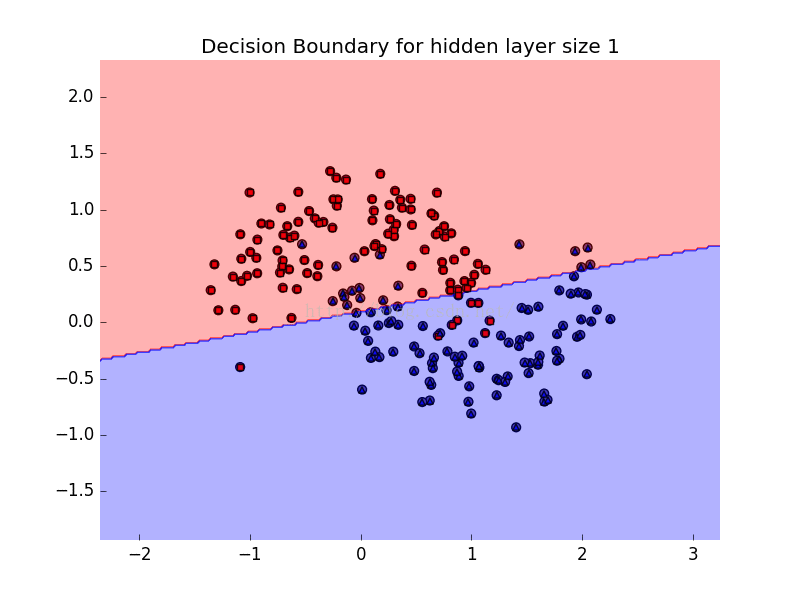
	plt.title("Decision Boundary for hidden layer size %d"%degree)
	plt.show()

原网址：http://python.jobbole.com/82208/，讲的非常好，但是那里的代码已经不能用了，感谢原作者

这里的代码能在python2.7，mlxtend-0.3.0下运行。

效果图如下：