COMSOL求解常微分方程

COMSOL Multiphysics多物理场仿真软件也提供了求救常微分方程（ODE）和偏微分方程（PDE）的接口,下面详细介绍一下。

（1）建立模型，选择模型向导–>零维–>数学–>全局常微分和微分代数方程(ge)，选择研究，选择瞬态，点击完成
（2）在组件下面可以看到刚刚添加的全局常微分和微分代数方程(ge)，在右边栏，全局方程那里输入需要求解的函数。

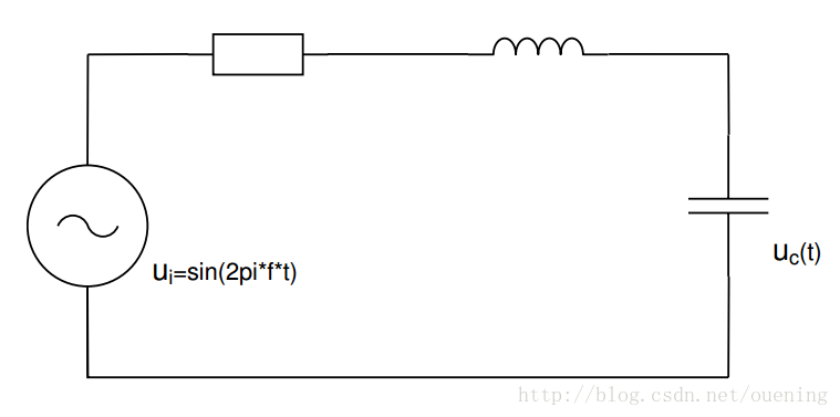
以上图电路实例来说，现有RLC串联电路，假设R、L、C的参数都为1,电容电压：$u_C(t)$，电容电流：$i(t)$，电感电压：$u_L(t)$，电阻电压：$u_R(t)$，输入电压$u_{in}=sin(2\pi ft)$则有下面的关系式：

$$\begin{equation} \begin{array}{rl} u_C(t) &= u_C(t) \\ i(t) &= C\frac{du_C(t)}{dt} \\ u_L(t) &= L\frac{di(t)}{dt}=LC\frac{du_C^2(t)}{dt^2} \\ u_R(t) &= Ri(t) = RC\frac{du_C(t)}{dt} \\ u_{in} &= u_C(t)+ u_L(t)+u_R(t) \end{array} \end{equation}$$
化简上式可得：
$$\frac{du_C^2(t)}{dt^2}+\frac{du_C(t)}{dt}+u_C(t)=u_{in}$$ ，换成常见的数学形式为
$$f''+f'+f=sin(2\pi ft)$$

要想在COMSOL求解该二阶微分方程，可以先用之前的方法在python里面求解，python代码如下：

from scipy.integrate import odeint
import numpy as np
import matplotlib.pyplot as plt
def f(y,t):
    dy1 = y[1]
    dy2 = np.sin(100*t)-y[0]-y[1]
    return [dy1,dy2]

t = np.linspace(0,20,3000)
# 初值[0,0]表示y(0)=0,y’(0)=0
# 返回y， 其中y[:,0]是y[0]的值 ，就是最终解 ，y[:,1]是y’(x)的值
y = odeint(f,[0,0],t)

l1, = plt.plot(t,y[:,0],label='y(0)')
#l2, = plt.plot(t,y[:,1],label='y(1)')

plt.legend()
plt.grid('on')
plt.show()

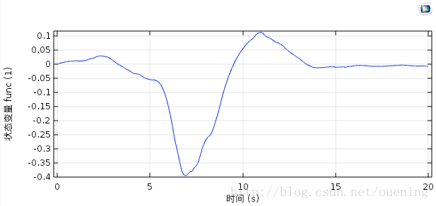
输出结果如下：

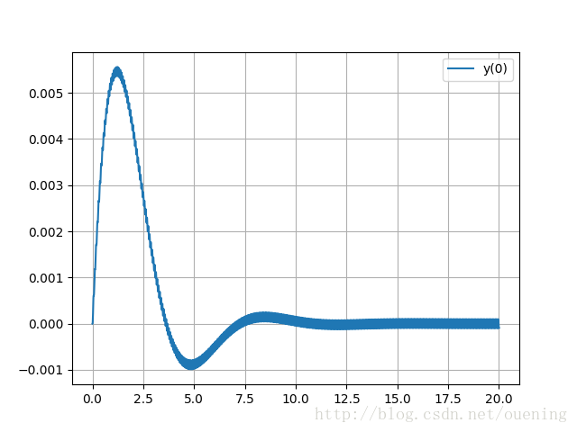
输入电源参数设置为$2\pi f=100$，初值设定为$y(0)=0$,$y'(0)=0$，由结果可知是一个衰减震荡的过程。

（3）步骤（2）得到的COMSOL设置结果如下：

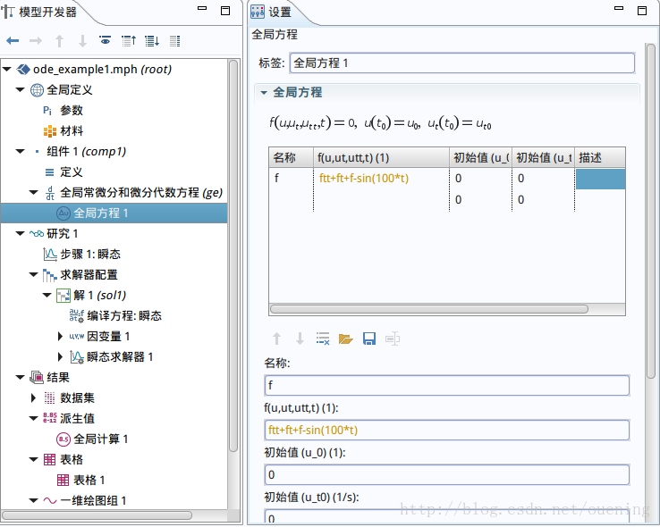
关于全局方程的书写官方原文如下：

In each column enter as follows:\
• Enter the Name of the state variable. This also defines time-derivative variables. If a state variable is called u, its
first and second time derivatives are ut and utt, respectively. These variables become available in all geometries.
Therefore the names must be unique.\
• Use the f(u,ut,utt,t) column to specify the right-hand side of the equation that is to be set equal to zero.
The software then adds this global equation to the system of equations. When solving the model, the value of
the state variable u is adapted in such a way that the associated global equation is satisfied. All state variables and
their time derivatives can be used as well as any parameters, global variables, and coupling operators with a scalar
output and global domain of definition in the f(u,ut,utt,t) column. The variables can be functions of the state
variables in the global equations. Setting an equation for a state is optional. The default value of 0 means that
the software does not add any additional condition to the model.\
• If the time derivative of a state variable appears somewhere in the model during a time-dependent solution, the
state variable needs an initial condition. Models that contain second time derivatives also require an initial value
for the first time derivatives of the state variables. Set these conditions in the third (Initial value (u_ 0)) and fourth (Initial value (u_t 0)) columns.\
• Enter comments about the state or the equation in the last column, Description.\
\emph{特别注意}：\
(1)方程名称是作为变量用于整个几何体的，因此不要在其他地方重复误用，本例的函数名为f，也可以是u,y,g,h以及func之类等\
(2)方程关于时间的一阶导和二阶导表达式写作：ft和ftt，这是以本例函数名称为f来说的，如果函数名为y,就是yt和ytt，如果函数名是func，就是funct和
functt；\

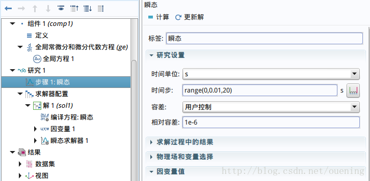
（4）按下图设置仿真步长和时间,range(0,0.01,20)意思是仿真时间0-20s（因为一开始建立模型的研究类型是瞬态），仿真步长0.01s：

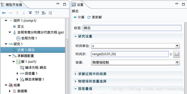
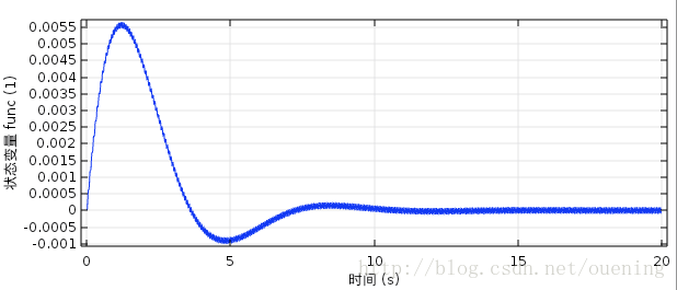
点击计算，发现结果与python求救不符合，结果如下图所示：

经过与前面python的结果对比，求解值比较小，数量级是$10^{-3}$，因此要修改COMSOL仿真配置中的容差，将\pmb{物理场控制}改为\pmb{用户控制}，设置容差为\pmb{1e-6}，设置和正确求解的最终结果如下图：

在COMSOL里自带的例子中，事先在\pmb{全局定义}设置了\pmb{参数}a,b,c，分别对应参数$\sigma$,$\rho$和$\beta$，方程设置如下：

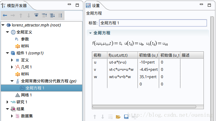
得到的结果和python求解的类似。