Deep Learning 练习一：Sparse Autoencoder

分类： 【Matlab】 2013-10-17 22:47  443人阅读  评论(0)  收藏  举报

目录(?)[+]

In this problem set, you will implement the sparse autoencoder algorithm, and show how it discovers that edges are a good representation for natural images. (Images provided by Bruno Olshausen.) The sparse autoencoder algorithm is described in the lecture notes found on the course website.

In the file sparseae_exercise.zip, we have provided some starter code in Matlab. You should write your code at the places indicated in the files ("YOUR CODE HERE"). You have to complete the following files: sampleIMAGES.m, sparseAutoencoderCost.m, computeNumericalGradient.m. The starter code in train.m shows how these functions are used.

Specifically, in this exercise you will implement a sparse autoencoder, trained with 8×8 image patches using the L-BFGS optimization algorithm.

A note on the software: The provided .zip file includes a subdirectory minFunc with 3rd party software implementing L-BFGS, that is licensed under a Creative Commons, Attribute, Non-Commercial license. If you need to use this software for commercial purposes, you can download and use a different function (fminlbfgs) that can serve the same purpose, but runs ~3x slower for this exercise (and thus is less recommended). You can read more about this in the Fminlbfgs_Details page.

train.m代码

[plain]  view plain copy

1. %% CS294A/CS294W Programming Assignment Starter Code  
2.   
3. %  Instructions  
4. %  ------------  
5. %   
6. %  This file contains code that helps you get started on the  
7. %  programming assignment. You will need to complete the code in sampleIMAGES.m,  
8. %  sparseAutoencoderCost.m and computeNumericalGradient.m.   
9. %  For the purpose of completing the assignment, you do not need to  
10. %  change the code in this file.   
11. %  
12. %%======================================================================  
13. %% STEP 0: Here we provide the relevant parameters values that will  
14. %  allow your sparse autoencoder to get good filters; you do not need to   
15. %  change the parameters below.  
16.   
17. visibleSize = 8*8;   % number of input units   
18. hiddenSize = 25;     % number of hidden units   
19. sparsityParam = 0.01;   % desired average activation of the hidden units.  
20.                      % (This was denoted by the Greek alphabet rho, which looks like a lower-case "p",  
21.              %  in the lecture notes).   
22. lambda = 0.0001;     % weight decay parameter         
23. beta = 3;            % weight of sparsity penalty term         
24.   
25. %%======================================================================  
26. %% STEP 1: Implement sampleIMAGES  
27. %  
28. %  After implementing sampleIMAGES, the display_network command should  
29. %  display a random sample of 200 patches from the dataset  
30.   
31. patches = sampleIMAGES;  
32. display_network(patches(:,randi(size(patches,2),200,1)),8);  
33.   
34.   
35. %  Obtain random parameters theta  
36. theta = initializeParameters(hiddenSize, visibleSize);  
37.   
38. %%======================================================================  
39. %% STEP 2: Implement sparseAutoencoderCost  
40. %  
41. %  You can implement all of the components (squared error cost, weight decay term,  
42. %  sparsity penalty) in the cost function at once, but it may be easier to do   
43. %  it step-by-step and run gradient checking (see STEP 3) after each step.  We   
44. %  suggest implementing the sparseAutoencoderCost function using the following steps:  
45. %  
46. %  (a) Implement forward propagation in your neural network, and implement the   
47. %      squared error term of the cost function.  Implement backpropagation to   
48. %      compute the derivatives.   Then (using lambda=beta=0), run Gradient Checking   
49. %      to verify that the calculations corresponding to the squared error cost   
50. %      term are correct.  
51. %  
52. %  (b) Add in the weight decay term (in both the cost function and the derivative  
53. %      calculations), then re-run Gradient Checking to verify correctness.   
54. %  
55. %  (c) Add in the sparsity penalty term, then re-run Gradient Checking to   
56. %      verify correctness.  
57. %  
58. %  Feel free to change the training settings when debugging your  
59. %  code.  (For example, reducing the training set size or   
60. %  number of hidden units may make your code run faster; and setting beta   
61. %  and/or lambda to zero may be helpful for debugging.)  However, in your   
62. %  final submission of the visualized weights, please use parameters we   
63. %  gave in Step 0 above.  
64.   
65. [cost, grad] = sparseAutoencoderCost(theta, visibleSize, hiddenSize, lambda, ...  
66.                                      sparsityParam, beta, patches);  
67.   
68. %%======================================================================  
69. %% STEP 3: Gradient Checking  
70. %  
71. % Hint: If you are debugging your code, performing gradient checking on smaller models   
72. % and smaller training sets (e.g., using only 10 training examples and 1-2 hidden   
73. % units) may speed things up.  
74.   
75. % First, lets make sure your numerical gradient computation is correct for a  
76. % simple function.  After you have implemented computeNumericalGradient.m,  
77. % run the following:   
78. checkNumericalGradient();  
79.   
80. % Now we can use it to check your cost function and derivative calculations  
81. % for the sparse autoencoder.    
82. numgrad = computeNumericalGradient( @(x) sparseAutoencoderCost(x, visibleSize, ...  
83.                                                   hiddenSize, lambda, ...  
84.                                                   sparsityParam, beta, ...  
85.                                                   patches), theta);  
86.   
87. % Use this to visually compare the gradients side by side  
88. disp([numgrad grad]);   
89.   
90. % Compare numerically computed gradients with the ones obtained from backpropagation  
91. diff = norm(numgrad-grad)/norm(numgrad+grad);  
92. disp(diff); % Should be small. In our implementation, these values are  
93.             % usually less than 1e-9.  
94.   
95.             % When you got this working, Congratulations!!!   
96.   
97. %%======================================================================  
98. %% STEP 4: After verifying that your implementation of  
99. %  sparseAutoencoderCost is correct, You can start training your sparse  
100. %  autoencoder with minFunc (L-BFGS).  
101.   
102. %  Randomly initialize the parameters  
103. theta = initializeParameters(hiddenSize, visibleSize);  
104.   
105. %  Use minFunc to minimize the function  
106. addpath minFunc/  
107. options.Method = 'lbfgs'; % Here, we use L-BFGS to optimize our cost  
108.                           % function. Generally, for minFunc to work, you  
109.                           % need a function pointer with two outputs: the  
110.                           % function value and the gradient. In our problem,  
111.                           % sparseAutoencoderCost.m satisfies this.  
112. options.maxIter = 400;    % Maximum number of iterations of L-BFGS to run   
113. options.display = 'on';  
114.   
115.   
116. [opttheta, cost] = minFunc( @(p) sparseAutoencoderCost(p, ...  
117.                                    visibleSize, hiddenSize, ...  
118.                                    lambda, sparsityParam, ...  
119.                                    beta, patches), ...  
120.                               theta, options);  
121.   
122. %%======================================================================  
123. %% STEP 5: Visualization   
124.   
125. W1 = reshape(opttheta(1:hiddenSize*visibleSize), hiddenSize, visibleSize);  
126. display_network(W1', 12);   
127.   
128. print -djpeg weights.jpg   % save the visualization to a file   

Step 1: Generate training set

The first step is to generate a training set. To get a single training example x, randomly pick one of the 10 images, then randomly sample an 8×8 image patch from the selected image, and convert the image patch (either in row-major order or column-major order; it doesn't matter) into a 64-dimensional vector to get a training example 

Complete the code in sampleIMAGES.m. Your code should sample 10000 image patches and concatenate them into a 64×10000 matrix.

To make sure your implementation is working, run the code in "Step 1" of train.m. This should result in a plot of a random sample of 200 patches from the dataset.

sampleIMAGES.m的代码：

[cpp]  view plain copy

1. function patches = sampleIMAGES()  
2. % sampleIMAGES  
3. % Returns 10000 patches for training  
4.   
5. load IMAGES;    % load images from disk   
6.   
7. patchsize = 8;  % we'll use 8x8 patches   
8. numpatches = 10000;  
9.   
10. % Initialize patches with zeros.  Your code will fill in this matrix--one  
11. % column per patch, 10000 columns.   
12. patches = zeros(patchsize*patchsize, numpatches);  
13.   
14. %% ---------- YOUR CODE HERE --------------------------------------  
15. %  Instructions: Fill in the variable called "patches" using data   
16. %  from IMAGES.    
17. %    
18. %  IMAGES is a 3D array containing 10 images  
19. %  For instance, IMAGES(:,:,6) is a 512x512 array containing the 6th image,  
20. %  and you can type "imagesc(IMAGES(:,:,6)), colormap gray;" to visualize  
21. %  it. (The contrast on these images look a bit off because they have  
22. %  been preprocessed using using "whitening."  See the lecture notes for  
23. %  more details.) As a second example, IMAGES(21:30,21:30,1) is an image  
24. %  patch corresponding to the pixels in the block (21,21) to (30,30) of  
25. %  Image 1  
26. imageCount=size(IMAGES,3);  
27. for patchNum = 1:10000  
28.     imageNum=randi(1,imageCount);  
29.     [rowNum colNum] = size(IMAGES(:,:,imageNum));  
30.     xPos = randi([1,rowNum-patchsize+1]);  
31.     yPos = randi([1,colNum-patchsize+1]);  
32.     patches(:,patchNum) = reshape(IMAGES(xPos:xPos+7,yPos:yPos+7,imageNum),64,1);   end  
33. end  
34. %% ---------------------------------------------------------------  
35. % For the autoencoder to work well we need to normalize the data  
36. % Specifically, since the output of the network is bounded between [0,1]  
37. % (due to the sigmoid activation function), we have to make sure   
38. % the range of pixel values is also bounded between [0,1]  
39. patches = normalizeData(patches);  
40. end  
41.   
42. %% ---------------------------------------------------------------  
43. function patches = normalizeData(patches)  
44.   
45. % Squash data to [0.1, 0.9] since we use sigmoid as the activation  
46. % function in the output layer  
47.   
48. % Remove DC (mean of images).   
49. patches = bsxfun(@minus, patches, mean(patches));  
50.   
51. % Truncate to +/-3 standard deviations and scale to -1 to 1  
52. pstd = 3 * std(patches(:));  
53. patches = max(min(patches, pstd), -pstd) / pstd;  
54.   
55. % Rescale from [-1,1] to [0.1,0.9]  
56. patches = (patches + 1) * 0.4 + 0.1;  
57.   
58. end  

Implementational tip: When we run our implemented sampleImages(), it takes under 5 seconds. If your implementation takes over 30 seconds, it may be because you are accidentally making a copy of an entire 512×512 image each time you're picking a random image. By copying a 512×512 image 10000 times, this can make your implementation much less efficient. While this doesn't slow down your code significantly for this exercise (because we have only 10000 examples), when we scale to much larger problems later this quarter with 10⁶ or more examples, this will significantly slow down your code. Please implement sampleIMAGES so that you aren't making a copy of an entire 512×512 image each time you need to cut out an 8x8 image patch.

Step 2: Sparse autoencoder objective

Implement code to compute the sparse autoencoder cost function J_sparse(W,b) (Section 3 of the lecture notes) and the corresponding derivatives of J_sparse with respect to the different parameters. Use the sigmoid function for the activation function, 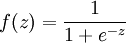. In particular, complete the code in sparseAutoencoderCost.m.

The sparse autoencoder is parameterized by matrices ,  vectors , . However, for subsequent notational convenience, we will "unroll" all of these parameters into a very long parameter vector θ with s₁s₂ + s₂s₃ +s₂ + s₃ elements. The code for converting between the (W⁽¹⁾,W⁽²⁾,b⁽¹⁾,b⁽²⁾) and the θ parameterization is already provided in the starter code.

Implementational tip: The objective J_sparse(W,b) contains 3 terms, corresponding to the squared error term, the weight decay term, and the sparsity penalty. You're welcome to implement this however you want, but for ease of debugging, you might implement the cost function and derivative computation (backpropagation) only for the squared error term first (this corresponds to setting λ = β = 0), and implement the gradient checking method in the next section to first verify that this code is correct. Then only after you have verified that the objective and derivative calculations corresponding to the squared error term are working, add in code to compute the weight decay and sparsity penalty terms and their corresponding derivatives.

Step 3: Gradient checking

Following Section 2.3 of the lecture notes, implement code for gradient checking. Specifically, complete the code incomputeNumericalGradient.m. Please use EPSILON = 10^-4 as described in the lecture notes.

We've also provided code in checkNumericalGradient.m for you to test your code. This code defines a simple quadratic function given by 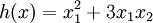, and evaluates it at the point x = (4,10)^T. It allows you to verify that your numerically evaluated gradient is very close to the true (analytically computed) gradient.

After using checkNumericalGradient.m to make sure your implementation is correct, next use computeNumericalGradient.m to make sure that yoursparseAutoencoderCost.m is computing derivatives correctly. For details, see Steps 3 in train.m. We strongly encourage you not to proceed to the next step until you've verified that your derivative computations are correct.

Implementational tip: If you are debugging your code, performing gradient checking on smaller models and smaller training sets (e.g., using only 10 training examples and 1-2 hidden units) may speed things up.

Step 4: Train the sparse autoencoder

Now that you have code that computes J_sparse and its derivatives, we're ready to minimize J_sparse with respect to its parameters, and thereby train our sparse autoencoder.

We will use the L-BFGS algorithm. This is provided to you in a function called minFunc (code provided by Mark Schmidt) included in the starter code. (For the purpose of this assignment, you only need to call minFunc with the default parameters. You do not need to know how L-BFGS works.) We have already provided code in train.m (Step 4) to call minFunc. The minFunc code assumes that the parameters to be optimized are a long parameter vector; so we will use the "θ" parameterization rather than the "(W⁽¹⁾,W⁽²⁾,b⁽¹⁾,b⁽²⁾)" parameterization when passing our parameters to it.

Train a sparse autoencoder with 64 input units, 25 hidden units, and 64 output units. In our starter code, we have provided a function for initializing the parameters. We initialize the biases  to zero, and the weights  to random numbers drawn uniformly from the interval , where n_in is the fan-in (the number of inputs feeding into a node) and n_out is the fan-in (the number of units that a node feeds into).

The values we provided for the various parameters (λ,β,ρ, etc.) should work, but feel free to play with different settings of the parameters as well.

Implementational tip: Once you have your backpropagation implementation correctly computing the derivatives (as verified using gradient checking in Step 3), when you are now using it with L-BFGS to optimize J_sparse(W,b), make sure you're not doing gradient-checking on every step. Backpropagation can be used to compute the derivatives of J_sparse(W,b) fairly efficiently, and if you were additionally computing the gradient numerically on every step, this would slow down your program significantly.

Step 5: Visualization

After training the autoencoder, use display_network.m to visualize the learned weights. (See train.m, Step 5.) Run "print -djpeg weights.jpg" to save the visualization to a file "weights.jpg" (which you will submit together with your code).

Results

To successfully complete this assignment, you should demonstrate your sparse autoencoder algorithm learning a set of edge detectors. For example, this was the visualization we obtained:

Our implementation took around 5 minutes to run on a fast computer. In case you end up needing to try out multiple implementations or different parameter values, be sure to budget enough time for debugging and to run the experiments you'll need.

Also, by way of comparison, here are some visualizations from implementations that we do not consider successful (either a buggy implementation, or where the parameters were poorly tuned):