180114 协方差矩阵几何含义与python-2D旋转变化

python matplotlib绘图设置坐标轴刻度、文本
matplotlib-ticker
旋转变换
协方差矩阵的几何解释-英文原文（翻墙可见）
协方差矩阵的几何解释-中文翻译

两个问题：
旋转变换时：θ是逆时针还是顺时针？
如果是逆时针，为何协方差矩阵分解得到的旋转矩阵的结果与实际结果差一个负号？

# -*- coding: utf-8 -*-
"""
Created on Sun Jan 14 12:44:40 2018

@author: brucelau
**两个问题**：
旋转变换时：θ是逆时针还是顺时针？
如果是逆时针，为何协方差矩阵分解得到的旋转矩阵的结果与实际结果差一个负号？
"""

import numpy as np
import matplotlib.pyplot as plt
from matplotlib.ticker import MultipleLocator, FormatStrFormatter

xmajorLocator   = MultipleLocator(1) #将x主刻度标签设置为20的倍数  
xmajorFormatter = FormatStrFormatter('%1.0f') #设置x轴标签文本的格式   
ymajorLocator   = MultipleLocator(1) #将y轴主刻度标签设置为0.5的倍数  
ymajorFormatter = FormatStrFormatter('%1.0f') #设置y轴标签文本的格式  

def data_vis(data_,title='abc'):
    lim = -15
    fig =  plt.figure()
    ax = fig.add_subplot(111)
    ax.scatter(data_[0,:],data_[1,:],s=1,c='k')
    ax.scatter(data_[0,1],data_[1,1],s=10,c='r')
    ax.scatter(data_[0,int(data_.shape[1]/2)],data_[1,int(data_.shape[1]/2)],s=10,c='b')
    ax.scatter(data_[0,-1],data_[1,-1],s=10,c='g')
    ax.set_xlim(-lim,lim)
    ax.set_ylim(-lim,lim)
    ax.grid()

    ax.xaxis.set_major_locator(xmajorLocator)  
    ax.xaxis.set_major_formatter(xmajorFormatter)   
    ax.yaxis.set_major_locator(ymajorLocator)  
    ax.yaxis.set_major_formatter(ymajorFormatter)
    ax.set_title(title)
#%%  emample test

#A = np.array([[3,2],[2,3]])
#print(A,'\n')

##evalue,evector = np.linalg.eig(A)
##print(evalue)
##print(evector)

#s,v,d = np.linalg.svd(A)
#print(s)
#print(v)
#print(d)

#print('The inverse of A is:\n',np.linalg.inv(s))
#R = s
#S = np.diag(np.sqrt(v))
#T = R*S
#%%
np.random.seed(0)
#%%
mu = np.array([0,0])
cov = np.identity(2)
data  = np.random.multivariate_normal(mu,cov,1000).T
data_sigma = np.cov(data)
# scale
m_scale = np.array([[4,0],[0,1]])
data_s = np.dot(m_scale,data)
data_s_sigma = np.cov(data_s)
#data_vis(data_scale)

# rotation after scale
theta = np.pi/6 #旋转变换时：θ是逆时针还是顺时针？加一个负号，则旋转分解结果与理论分析一致，否则相反
m_rotation = np.array([[np.cos(theta),-np.sin(theta)],[np.sin(theta),np.cos(theta)]])
data_r = np.dot(m_rotation,data_s)
#data_vis(data_r)

# scale and rotation
m_sc = np.dot(m_rotation,m_scale)
data_rc = np.dot(m_sc,data)
#data_vis(data_rc)

# analysis
data_rc_sigma = np.cov(data_rc) 
V,L,V_ = np.linalg.svd(data_rc_sigma)
print('After SVD U is\n',V)
print('After SVD ∑ is\n',L)
print('After SVD V is\n',V_,'\n')

R = V
S = np.diag(np.sqrt(L))
T = R*S
print('The Pred-Rotation matrix is:\n',R)
print('The True-Rotation matrix is:\n',m_rotation,'\n')
print('The Pred-Scaling matrix is :\n',S)
print('The True-Scaling matrix is :\n',m_scale)

#%% plot data distribution
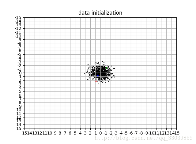
data_vis(data,title='data initialization')
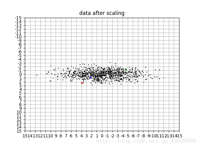
data_vis(data_s,title='data after scaling')
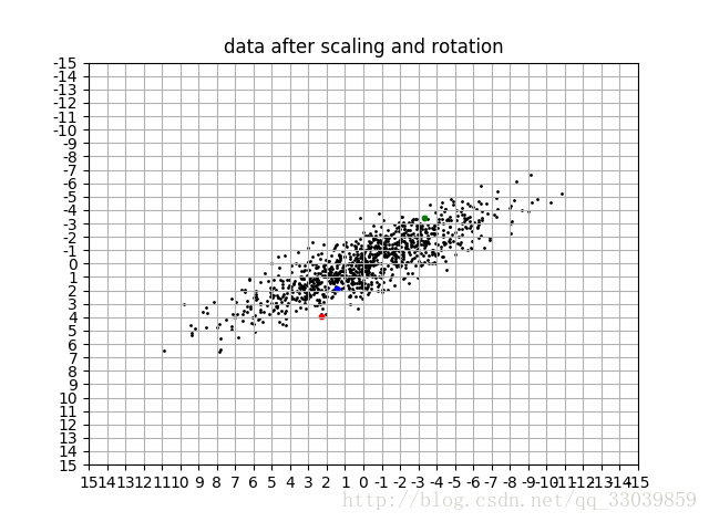
data_vis(data_rc,title='data after scaling and rotation')

After SVD U is
[[-0.8678919 -0.49675311]
[-0.49675311 0.8678919 ]]
After SVD ∑ is
[ 15.2062307 0.96456971]
After SVD V is
[[-0.8678919 -0.49675311]
[-0.49675311 0.8678919 ]]

---

The Pred-Rotation matrix is:
[[-0.8678919 -0.49675311]
[-0.49675311 0.8678919 ]]
The True-Rotation matrix is:
[[ 0.8660254 -0.5 ]
[ 0.5 0.8660254]]

---

The Pred-Scaling matrix is :
[[ 3.89951673 0. ]
[ 0. 0.9821251 ]]
The True-Scaling matrix is :
[[4 0]
[0 1]]