


- 求解非线性方程组。
比如求解:
cos(a) = 1 - d^2 / (2*R^2) L = a * r
from math import cos
from scipy import optimize
def f(x):
    d = 140
    l = 156
    a, r = x.tolist()
    return [
        cos(a) - 1 + (d*d)/(2*r*r),
        l - r * a
    ]
result = optimize.fsolve(f,[1, 1])
print result
print f(result)
[  1.5940638   97.86308398]   #结果
[4.596323321948148e-14, 2.7682744985213503e-11]  #误差
传入的参数是雅克比矩阵提高运算速度:
例如三个参数三个未知数:
在本例中:
from math import cos,sin
from scipy import optimize
def f(x):
    d = 140
    l = 156
    a, r = x.tolist()
    return [
        cos(a) - 1 + (d*d)/(2*r*r),
        l - r * a
    ]
def j(x):
    d = 140
    l = 156
    a, r = x.tolist()
    return [
        [-sin(a), (d*d)/4*r],
        [-r,-a]
    ]
result = optimize.fsolve(f, [1, 1], fprime=j)
print result
print f(result)

[  2.5761077   60.55647445]
[0.8280923609129465, 9.817000545808696e-09]
当未知数很多时计算雅克比矩阵可以明显提高速度
2.统计(stats模块)
连续随机变量对象都有如下方法:
- rvs:对随机变量进行随机取值,可以通过size参数指定输出的数组的大小。
- pdf:概率密度函数
- cdf:分布函数。F(x)表示随机变量的取值 <x <script type="math/tex" id="MathJax-Element-1">
- sf:随机变量的生存函数1-cdf(t)
- ppf:累积分布函数的反函数
- stat:计算随机变量的期望和方差
- fit:拟合,找到最适合取样数据的概率密度函数的系数。
import numpy as np
from scipy import stats
X = stats.norm(loc=1.0, scale=2.0)
x = X.rvs(size=10000)
pdf, t = np.histogram(x, bins=100, normed=True)#将x的取值范围分成100个区间,统计中的每个值落入区间的次数。
                                            #返回值pdf是落入每个区间的次数,由于normed未True,因此pdf是正规化后的结果,
                                            #应与概率密度曲线一致
                                            #t表示区间,包含起点和终点因此长度为101,然后计算中间值

t = (t[:-1] + t[1:]) * 0.5                   #每个区间的起点和终点相加

cdf = np.cumsum(pdf) * (t[1] -t[0])          #计算分布函数
sum = 0

p_error = pdf - X.pdf(t)
c_error = cdf - X.cdf(t)
print "max pdf error{}, max cdf error:{}".format(np.abs(p_error).max, np.abs(c_error).max())

max pdf error<built-in method max of numpy.ndarray object at 0x0000000004E2A8A0>, max cdf error:0.0156576760085
离散概率分布有如:
import numpy as np
import matplotlib.pyplot as plt
from scipy import stats
x = range(1, 7)
p = (0.4, 0.2, 0.1, 0.1, 0.1, 0.1)
dice = stats.rv_discrete(values=(x, p))  #创建随机变量
np.random.seed(42)
samples = dice.rvs(size=(2000, 50))
sample_mean = np.mean(samples, axis=1)
_, bins, step = plt.hist(sample_mean, bins=100, normed=True, histtype="step",label=u"直方图统计")
'''
_: 直方图向量,是否归一化由参数normed设定

bins: 返回各个bin的区间范围

step: 返回每个bin里面包含的数据,是一个list
'''
kde = stats.kde.gaussian_kde(sample_mean)
x = np.linspace(bins[0], bins[-1], 100)
plt.plot(x, kde(x), label=u"核密度估计")
mean, std = stats.norm.fit(sample_mean)
plt.plot(x, stats.norm(mean, std).pdf(x),alpha=0.8, label=u"正态分布拟合")
plt.legend()
plt.savefig("C:\\figure1.png")
3.二项分布、泊松分布、伽马分布
- 二项分布
f(k,n,p)n次试验每次成功的概率都是p成功k次的概率。
投掷一次骰子,出现6的概率是 1/6 ,试验次数是5次,下面计算k为0到6时对应的概率
print stats.binom.pmf(range(6), 5, 1/6.0)
[  4.01877572e-01   4.01877572e-01   1.60751029e-01   3.21502058e-02 3.21502058e-03   1.28600823e-04]
在二项分布中如果n很大,p很小可以近似为泊松分布,
λ=np
,
f(k,λ)=e−λk!
import numpy as np
from scipy import stats
import pylab as pl

_lambda = 10
pl.figure(figsize=(10,4))
for i, time in enumerate([1000, 50000]):
    t = np.random.uniform(0, time, size=_lambda * time)  #产生_lambda*time个(0,time)的数
    count, time_edges = np.histogram(t, bins=time, range=(0, time))#统计时间发生次数
    dist, count_edges = np.histogram(count, bins=20, range=(0,20), normed=True)#统计20秒内的概率分布,normed为True结果和概率密度相等
    x = count_edges[:-1]
    poisson = stats.poisson.pmf(x, _lambda)
    pl.subplot(121+i)
    pl.plot(x, dist, "-o", lw=2, label=u"统计结果")
    pl.plot(x, poisson, "->", lw=2, label=u"泊松分布", color="red")
    pl.xlabel(u"次数")
    pl.ylabel(u"概率")
    pl.title(u"time = %d" % time)
    pl.legend(loc="lower center")

pl.show()
- 伽马分布
from scipy import stats
import numpy as np
import pylab as pl


parameters = [(1,2),(2,2),(3,2),(5,1),(9,0.5)]
x = np.linspace(0, 20, 1000)

for p in parameters:
    y = stats.gamma.pdf(x, p[0], scale=p[1])
    pl.plot(x, y, label="k=%d, theta=%.1f" % (p))
pl.legend()
pl.show()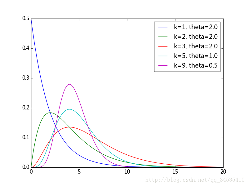
- 学生t-分布与t-检验
从均值为 u 的正态分布中,抽取n个值得样本,计算样本均值x¯ 和样本方差 s2 ,则 t=x¯−us/n√ ,符合df=n-1的学生t-分布。t值是抽选的样本的平均值与整体样本的期望值之差经过正规化后的数值,可以用来描述抽取的样本与整体样本之间的差异
from scipy import stats
import numpy as np
import matplotlib.pyplot as pl
mu = 0.0
n = 10
samples = stats.norm(mu).rvs(size=(100000, n))  #创建一个正态分布数组
t_samples = (np.mean(samples, axis=1) - mu) / np.std(samples, ddof=1, axis=1)*n**0.5#计算t值

sample_dict, x = np.histogram(t_samples, bins=100, density=True)
x = 0.5 * (x[:-1] + x[1:])
t_dist = stats.t(n-1).pdf(x)

print np.max(np.abs(sample_dict - t_dist))
pl.plot(x, sample_dict,  "*", lw=1, label=u"统计结果")
pl.plot(x, t_dist, lw=2, label=u"伽玛分布", color="red")


pl.legend()
pl.savefig("c:\\figure1.png")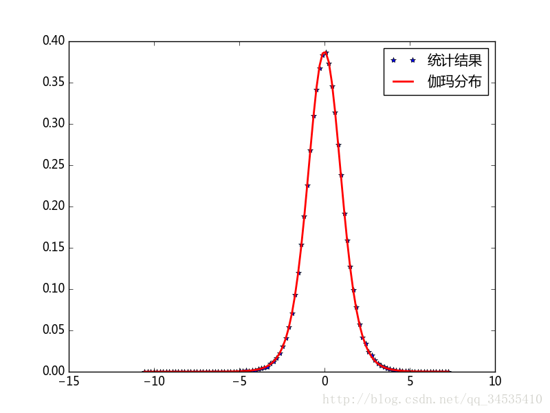
t-检验
import numpy as np
from scipy import stats
from matplotlib import pyplot as plt
n = 30
np.random.seed(30)
s = stats.norm.rvs(loc=1, scale=0.8, size=n)
t = (np.mean(s) - 0.5) / (np.std(s, ddof=1) / np.sqrt(n))
print t,stats.ttest_1samp(s, 0.5)
#stats.ttest_1samp()返回值的第一个参数是前面公式计算得到的t值,第#二个值被称为p值。当p值小于0.05时,通常我们认为假设不成立。
#假设期望是0.05
plt.savefig("c:\\figure1.png")

2.70076245943 Ttest_1sampResult(statistic=2.7007624594283199, pvalue=0.011429188829275502)  #拒绝假设
import numpy as np
from scipy import stats
from matplotlib import pyplot as plt
n = 30
np.random.seed(30)
s = stats.norm.rvs(loc=1, scale=0.8, size=n)
x = np.linspace(-5, 5, 500)
y = stats.t(n-1).pdf(x)
plt.plot(x, y, lw=2)
t, p = stats.ttest_1samp(s, 0.5)
mask = x > np.abs(t)
plt.fill_between(x[mask], y[mask], color="red", alpha=0.5)
mask = x < -np.abs(t)
plt.fill_between(x[mask], y[mask], color="red", alpha=0.5)
plt.axhline(color="k", lw=0.5)
plt.xlim(-5, 5)
plt.savefig("c:\\figure1.png")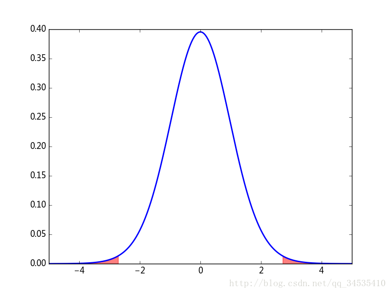
- 如果s1和s2是两个来自正态分布总体的样本,可以通过ttest_ind()检测两个样本的均值是否存在差异,equal_var参数为True和False代表有无差异。
import numpy as np
from scipy import stats
from matplotlib import pyplot as plt
np.random.seed(42)
s1 = stats.norm.rvs(loc=1, scale=1.0, size=20000)
s2 = stats.norm.rvs(loc=1.5, scale=0.5, size=20000)
s3 = stats.norm.rvs(loc=1.5, scale=0.5, size=25000)
print stats.ttest_ind(s1, s2, equal_var=False)
print stats.ttest_ind(s3, s2, equal_var=True)

Ttest_indResult(statistic=-61.80547575000832, pvalue=0.0)
Ttest_indResult(statistic=1.9233614532869769, pvalue=0.054440973916105452)- 卡方分布和卡方检验
k个独立的标准正态分布变量的平方和服从自由度为k的卡方分布。
import numpy as np
from scipy import stats
from matplotlib import pyplot as plt
a = np.random.normal(size=(300000, 4))
cs = np.sum(a**2, axis=1)
sample_dict, bins = np.histogram(cs, bins=100, range=(0, 20), density=True)
x = 0.5 * (bins[:-1] + bins[1:])
chi2_dist = stats.chi2.pdf(x, 4)
plt.plot(x, sample_dict, lw =2, label=u"数据统计")
plt.plot(x, chi2_dist, color='red', lw=2, label=u"卡方分布")
plt.legend()
plt.savefig("c:\\figure1.png")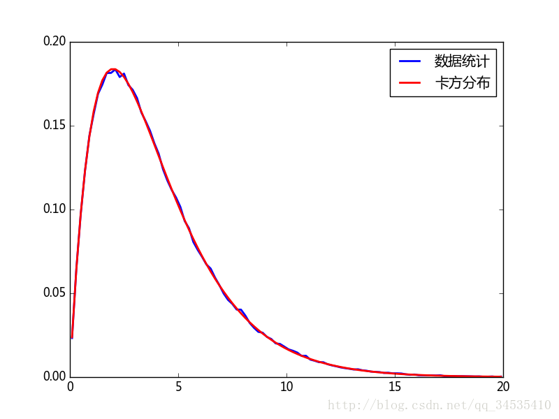
例子:
袋子里有5种颜色的球,抽到每种球的概率相同,从中选N次,并统计每种颜色的次数
Oi
则下面的
χ2
符合自由度为4的卡方分布,其中
E=N/5
为每种球被抽选的期望次数。
χ2=∑i=1kOi−EE
import numpy as np
from scipy import stats
from matplotlib import pyplot as plt
repeat_count = 60000
n, k = 100, 5
np.random.seed(42)
ball_ids = np.random.randint(0, k, size=(repeat_count, n))
#创建从0到5的随机数,第0轴表示试验次数,第1轴表示抽取的100个球的编号。
counts = np.apply_along_axis(np.bincount, 1, ball_ids, minlength=k)
#使用bincount()统计试验中每个编号出现的次数,为保证每行统计结果相同
#设置minlength=5
#apply_along_axis()对第1轴上的数据循环调用bincount()
cs2 = np.sum((counts - n/k)**2.0/(n/k), axis=1)
#计算统计量
k = stats.kde.gaussian_kde(cs2)
#计算cs2的分布情况
x = np.linspace(0, 10, 200)
plt.plot(x, stats.chi2.pdf(x, 4), lw=2, label=u'$\chi ^{2}$分布')
plt.plot(x, k(x), lw=2, color='red', alpha=0.6, label=u"样本分布")
plt.legend(loc="best")
plt.xlim(0, 10)
plt.show()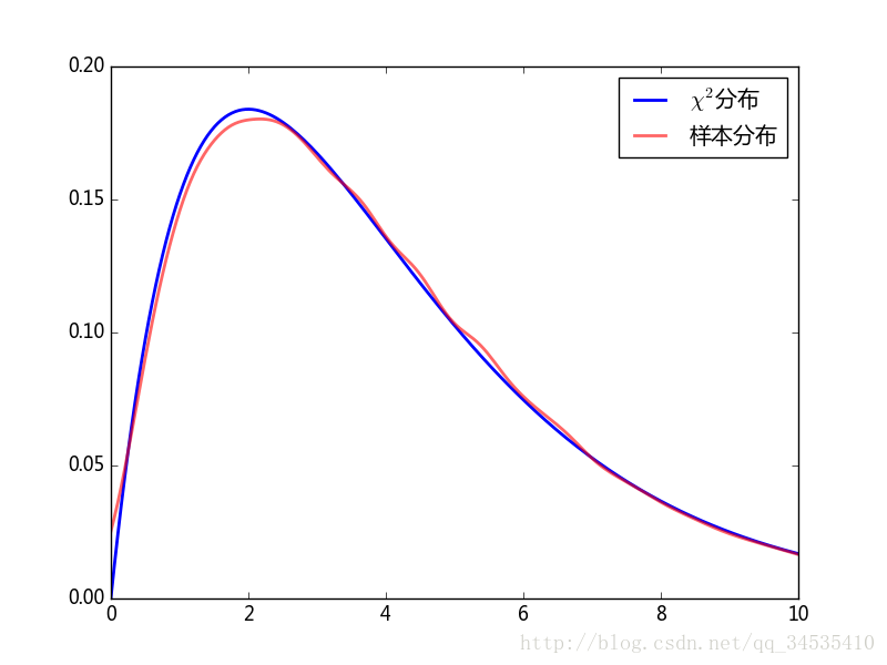
- 卡方检验可以用来评估观测值与理论值的差异是否只是因为随机误差造成的。在下面的例子中,袋子中各种颜色的球按照probablities参数指定的概率分布,choose_balls(probabilities,size)从袋中选择size次并返回每种球
from scipy import stats
import numpy as np
def choose_balls(probabolities, size):
    r = stats.rv_discrete(values=(range(len(probabolities)), probabolities))
    s = r.rvs(size=size)
    counts = np.bincount(s)
    return counts
#得到选择每个球的次数
np.random.seed(42)
counts1 = choose_balls([0.18, 0.24, 0.25, 0.16, 0.17], 400)
counts2 = choose_balls([0.2] * 5, 400)
chi1, p1 = stats.chisquare(counts1)
'''进行卡方检验,参数为每种球被选中的次数的列表,如果没有设置检验的目标概率,就测试他们是否符合均匀分布。有结果可知第一个袋中p值为0.02,意思如果真是均匀分布得到结果1的概率是2%,因此可以推翻假设袋中的球是均匀分布的。*假设只能用来否定。*
'''
chi2, p2 = stats.chisquare(counts2)
print "ch1 =", chi1, "p1=", p1
print "ch2 =", chi2, "p2=", p2

ch1 = 11.375 p1= 0.0226576012398
ch2 = 2.55 p2= 0.635705452704
卡方检验用于二维数据
| ” “ | 右手 | 左手 |
|---|---|---|
| 男性 | 43 | 9 |
| 女性 | 44 | 4 |
假设性别与惯用手之间不存在关系,即男性与女性管用左右手的概率相同。
from scipy import stats
table = [[43, 9], [44, 4]]
chi2, p, dof, expected = stats.chi2_contingency(table)
print p

0.300384770391
由于p为0.3,因此不能否定假设
4.最小二乘拟合
在python的optimize模块中,可以使用leastq()对数据进行最小二乘拟合计算。leastsq()只需将计算误差的函数和待确定参数的初始值传递给他即可。
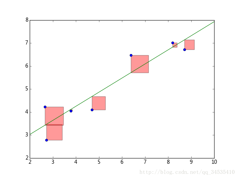
拟合直线
import numpy as np
from scipy.optimize import leastsq

X = np.array([ 8.19,  2.72,  6.39,  8.71,  4.7 ,  2.66,  3.78])
Y = np.array([ 7.01,  2.78,  6.47,  6.71,  4.1 ,  4.23,  4.05])
def residuals(p):
    k, b = p
    return Y - (k*X + b)
#计算以p为参数的直线和原始数据之间的误差
r = leastsq(residuals, [1, 3])#使得输出数组的平方和最小,初始值是【1,3】
k, b = r[0]
print k, b
#下面是绘图部分
import pylab as pl
from matplotlib.patches import Rectangle

pl.plot(X, Y, "o")
X0 = np.linspace(2, 10, 3)
Y0 = k*X0 + b
pl.plot(X0, Y0)

for x, y in zip(X, Y):
    y2 = k*x+b
    rect = Rectangle((x,y), abs(y-y2), y2-y, facecolor="red", alpha=0.4)
    pl.gca().add_patch(rect)

pl.gca().set_aspect("equal")
pl.show()
拟合正弦曲线
import numpy as np
from scipy import optimize
from matplotlib import pyplot as plt
def func(x, p):
    '''
    数据拟合所用的函数: A*sin(2*pi*k*x + theta)
   '''
    A, k, theta = p
    return A*np.sin(2*np.pi*k*x + theta)
def residuals(p, y, x):
    '''
    实验数据x,y和拟合函数之间的差,p为拟合需要找到的系数
    '''
    return y - func(x, p)
x = np.linspace(0, 2*np.pi, 100)
A, k, theta = 10, 0.34, np.pi/6   #真实数据的参数
y0 = func(x, [A, k, theta])       #真实数据
#加入噪声
np.random.seed(0)
y1 = y0 + 2 * np.random.randn(len(x))
p0 = [7, 0.40, 0]
#拟合
plsq = optimize.leastsq(residuals, p0, args=(y1, x))
print plsq[0]
plt.plot(x, y1, "o", label=u"带噪声的实验数据", alpha=0.5)
plt.plot(x, func(x, plsq[0]), "b-", label=u"拟合的曲线")
plt.plot(x, func(x,p0), 'g--',lw=2, label=u"真实曲线")
plt.legend()

plt.savefig("C:\\figure1.png")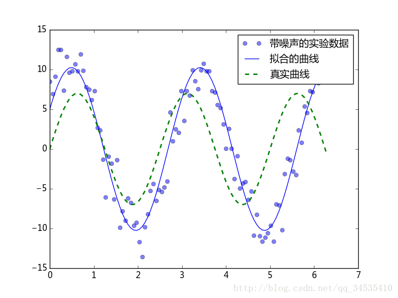
optimize库中的cure_fit()参数也可以进行拟合5、计算函数局域最小值
import scipy.optimize as opt
import numpy as np
import sys

points = []

def f(p):
    x, y = p
    z = (1-x)**2 + 100*(y-x**2)**2
    points.append((x, y, z))
    return z

def fprime(p):
    x, y = p
    dx = -2 + 2*x - 400*x*(y - x**2)
    dy = 200*y - 200*x**2
    return np.array([dx, dy])


init_point =(-2, -2)

try:
    method = sys.argv[1]
except:
    method = "fmin_bfgs"

fmin_func = opt.__dict__[method]
if method in ["fmin", "fmin_powell"]:
    result = fmin_func(f, init_point)    #参数为目标函数和初始值
elif method in ["fmin_cg", "fmin_bfgs", "fmin_l_bfgs_b", "fmin_tnc"]:
    result = fmin_func(f, init_point, fprime)    #参数为目标函数、初始值和导函数
elif method in ["fmin_cobyla"]:
    result = fmin_func(f, init_point, [])
else:
    print "fmin function not found"
    sys.exit(0)

### 绘图部分
import pylab as pl
p = np.array(points)
xmin, xmax = np.min(p[:, 0])-1, np.max(p[:, 0])+1
ymin, ymax = np.min(p[:, 1])-1, np.max(p[:, 1])+1
Y, X = np.ogrid[ymin:ymax:500j,xmin:xmax:500j]
Z = np.log10(f((X, Y)))
zmin, zmax = np.min(Z), np.max(Z)
pl.imshow(Z, extent=(xmin, xmax, ymin, ymax), origin="bottom", aspect="auto")
pl.plot(p[:, 0], p[:, 1])
pl.scatter(p[:, 0], p[:, 1], c=range(len(p)))
pl.xlim(xmin, xmax)
pl.ylim(ymin, ymax)
pl.savefig("C:\\figure1.png")
6.线性代数
奇异值分解
from scipy import linalg
import numpy as np
import matplotlib.pyplot as pl
r, g, b = np.rollaxis(pl.imread("C:\\timg.jpg"), 2).astype(float)
img = 0.289 * r + 0.5870 * g + 0.1140 * b
u, s, v = linalg.svd(img)   #s对应奇异值
def composite(u, s, v, n):
    return np.dot(u[:, :n], s[:n, np.newaxis] * v[:n, :])
img10 = composite(u, s, v, 10)
img20 = composite(u, s, v, 20)
img50 = composite(u, s, v, 50)
pl.subplot(221)
pl.imshow(img)
pl.subplot(222)
pl.imshow(img10)
pl.subplot(223)
pl.imshow(img20)
pl.subplot(224)
pl.imshow(img50)
pl.savefig("c:\\figure1.png")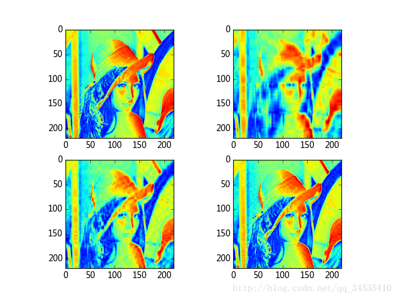
7.数值积分
- 计算半径为1的圆的面积:
from scipy import integrate
def half_circle(x):
    return (1 - x**2)**0.5
pi_half, err = integrate.quad(half_circle, -1, 1)
print pi_half*2
3.14159265359
quad()提供了dblquad()模块计算二重积分,tplquad()模块计算三重积分。计算 x2+y2+z2=1 的球体的体积。
半球体体积的二重积分:
∫1−1∫1−x2√−1−x2√1−x2−y2−−−−−−−−−√dydx
from scipy import integrate
def half_circle(x):
    return (1 - x**2)**0.5
def half_sphere(x, y):
    return (1-x**2-y**2)**0.5

v, err = integrate.dblquad(half_sphere, -1, 1, lambda x:-half_circle(x), lambda x:half_circle(x))
print v,err
2.09439510239 1.00023567207e-09
7.信号处理
- 中值滤波:中值滤波能比较有效的消除声音信号中的瞬间噪声或者图像中的斑点噪声。在signal模块中,medfilt()对一维信号进行中值滤波,二medfit2d()对二维信号进行中值滤波。在scipy.ndimage有针对多维图像的中值滤波器。
import numpy as np
from matplotlib import pyplot as plt
from scipy import signal
t = np.arange(0, 20, 0.1)
x = np.sin(t)
x[np.random.randint(0, len(t), 20)] +=np.random.standard_normal(20)*0.6
x2 = signal.medfilt(x, 5)#5是窗口值得大小,必须为奇数
plt.plot(t, x,color="red",lw=3,alpha =0.4, label=u"带噪声")
plt.plot(t, x2,  lw=1, label=u"中值滤波后")
plt.legend()
plt.savefig("c:\\figure1.png")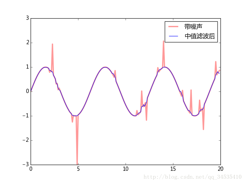
8.插值
import numpy as np
from matplotlib import pyplot as plt
from scipy import interpolate
#决定插值曲线的数据点有11个,插值之后的数据点有101个
y = np.sin(x)
xnew = np.linspace(0, 10, 101)
plt.plot(x, y, 'ro')
for kind in ['nearest', 'zero', 'slinear', 'quadratic']:
'''
zero、nearest:阶梯插值
slinear、linear:线性插值
quadratic、cubic:二阶和三阶B样条插值

'''
    f = interpolate.interp1d(x, y, kind=kind)#interpld可以计
    #算x的取值范围内的任意点的函数值
    ynew = f(xnew)
    plt.plot(xnew, ynew, label=str(kind))
plt.legend()
#plt.show()
plt.savefig("c:\\figure1.png")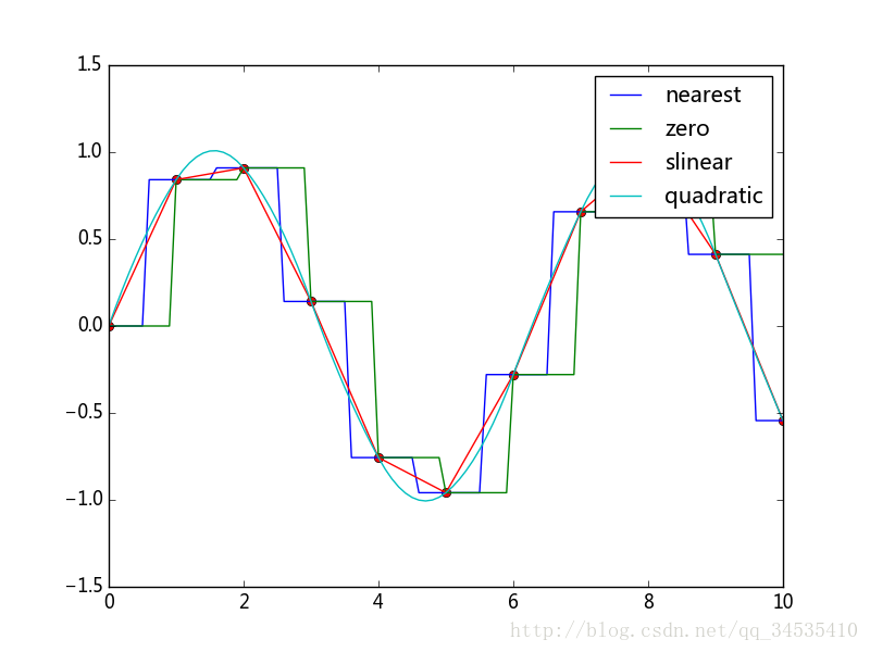
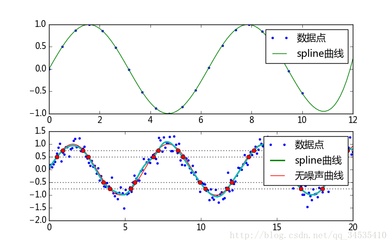
UnivariateSpline可以进行外推和拟合曲线
UnivariateSpline(x, y, w = None, bbox=[None, Nne], k=3, s=None]
x必须是递增的序列
w是每个数据点指定的权重值
k为样条曲线的阶数
s是平滑系数,s=0时曲线经过每一个点。
import numpy as np
from matplotlib import pyplot as plt
from scipy import interpolate
x1 = np.linspace(0, 10, 20)
y1 = np.sin(x1)
sx1 = np.linspace(0, 12, 100)
sy1 = interpolate.UnivariateSpline(x1, y1, s=0)(sx1)
#外推运算使得输入数据x的值没有大于10的点但是能计算出在10到12之间的数值
x2 = np.linspace(0, 20, 200)
y2 = np.sin(x2) + np.random.standard_normal(len(x2))*0.2
sx2 = np.linspace(0, 20, 2000)
spline2 = interpolate.UnivariateSpline(x2, y2, s=8)
sy2 = spline2(sx2)
plt.figure(figsize=(8, 5))
plt.subplot(211)
plt.plot(x1, y1, ".", label=u"数据点")
plt.plot(sx1, sy1, label=u"spline曲线")
plt.legend()
plt.subplot(212)
plt.plot(x2, y2, ".", label=u"数据点")
plt.plot(sx2, sy2, linewidth=2, label=u"spline曲线")
plt.plot(x2, np.sin(x2), label=u"无噪声曲线")
plt.legend()
#计算曲线和横线的交点
def root_at(self, v):
    coeff = self.get_coeffs()
    coeff -= v
    try:
        root = self.roots()
        return root
    finally:
        coeff += v
interpolate.UnivariateSpline.roots_at = root_at
plt.plot(sx2, sy2, lw = 2, label=u"spline曲线")
ax = plt.gca()
for level in [0.5, 0.75, -0.5, -0.75]:
    ax.axhline(level, ls=":", color="k")
    xr = spline2.roots_at(level)
    plt.plot(xr, spline2(xr), "ro")
#plt.show()
plt.savefig("c:\\figure1.png")
- 参数插值
x和y的数值由参数t控制。 x=f(t),y=f(t),
import numpy as np
from matplotlib import pyplot as plt
from scipy import interpolate
x = np.random.rand(10)
y = np.random.rand(10)
np.random.shuffle(y)
plt.plot(x, y, 'o')
for s in (0, 1e-4):
    tck, t = interpolate.splprep([x, y], s=s)
    #首先调用splprep(),其第一个参数为一组一维数组,每个数组是各点在
    #对应轴上的坐标s为平滑系数。splprep()返回两个对象,其中tck是一个
    #元祖,它包含了插值曲线的所有信息,t是自动计算出参数曲线的参数数组。
#调用splev()进行插值运算,其第一个参数为一个新的参数数组,第二个为
#splprep()返回的第一个对象。
    if s == 0:
        plt.plot(xi, yi, lw=1, label=u"s=%g" %s)
    else:
        plt.plot(xi, yi, lw=3, alpha=0.4, label=u"s=%g" %s)
plt.legend()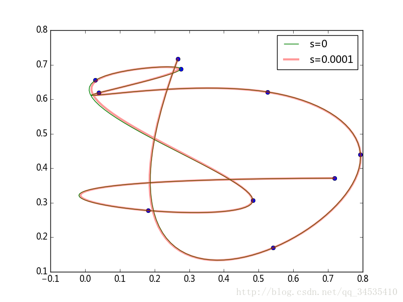
- 单调插值pchip():保证曲线的所有最值都出现在数据点之上
import numpy as np
from matplotlib import pyplot as plt
from scipy import interpolate
x = [0, 1, 2, 3, 4, 5]
y = [1, 2, 1.5, 2.5, 3, 2.5]
xs = np.linspace(x[0], x[-1], 100)
curve = interpolate.pchip(x, y)
ys = curve(xs)
plt.plot(xs, ys, label=u"pchip")
plt.plot(x, y, "o")
plt.legend()
plt.grid()
plt.margins(0.1, 0.1)
plt.show()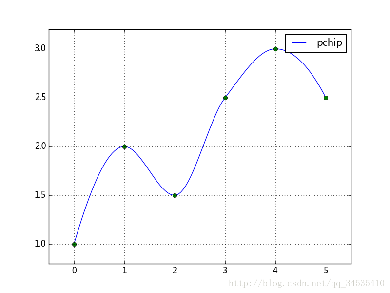
多维插值可以使用interp2d()、griddata()
- 径向基函数插值
所谓径向基函数,是指函数值只与某特定点的距离相关的一类函数 Φ(||X−Xi||) ,其中 xi 是某给定取样点的坐标。使用这些 Φ 函数可进食表示 N 维空间中的函数:
y(x)=∑Ni=1wiΦ(||X−Xi||)
下面的例子在以为插值中使用三种 Φ 函数multiquadric、gaussian、和linear
import numpy as np
from matplotlib import pyplot as plt
from scipy.interpolate import Rbf
x = np.array([-1, 0, 2.0, 1.0])
y = np.array([1.0, 0.3, -0.5, 0.8])
funcs = ['multiquadric', 'gaussian', 'linear']
nx = np.linspace(-3, 4, 100)


for fname in funcs:
    rbfs = Rbf(x, y, function=fname)
    rbf_ys = rbfs(nx)
    plt.plot(nx, rbf_ys, label=fname)
plt.legend()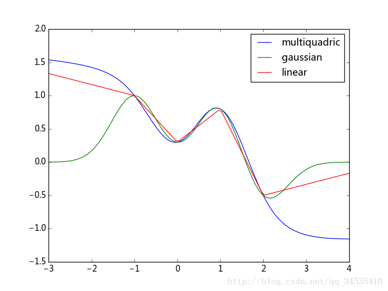
9.稀疏矩阵
scipy.sparse中提供了多种表示稀疏矩阵的格式,scipy.sparse.linalg提供了针对这些矩阵进行线性代数运算的函数,scipy.sparse.scgraph提供了对用稀疏矩阵表示的图进行搜索的函数
from scipy import sparse
a = sparse.dok_matrix((10, 5))
for i in range(10):
    for j in range(5):
        if i<=j:
            a[i,j] = i+j
print a.keys()
print a.values()
#dok_martix使用字典保存矩阵,键是行列的信息,对应的值是对应的矩阵中位于(行,列)的元素值。

b = sparse.lil_matrix((10, 5))
b[2, 3] = 1
b[3, 4] = 2
b[3, 2] = 3
print b.data
print b.rows
#lil_matrix使用两个列表保存矩阵,data保存每行中的非零元素,rows保存非零元所在的列
'''
另外还有coo_matrix采用三个数组row,col,和data保存非零元素的信息。这三个数组长度相同。coo_matrix
一旦创建后不支持元素的存取和增删
支持重复元素,同一行列有几个元素出现,转换为矩阵式求和输出。

'''

row = [2, 3, 3, 2]
col = [3, 4, 2, 3]
data = [1, 2, 3, 10]
c = sparse.coo_matrix((data, (row, col)), shape=(5, 6))
print c.toarray()

[(0, 1), (1, 2), (1, 3), (3, 3), (2, 2), (4, 4), (1, 4), (0, 2), (2, 3), (0, 4), (2, 4), (0, 3), (3, 4), (1, 1)]
[1.0, 3.0, 4.0, 6.0, 4.0, 8.0, 5.0, 2.0, 5.0, 4.0, 6.0, 3.0, 7.0, 2.0]
[[] [] [1.0] [3.0, 2.0] [] [] [] [] [] []]
[[] [] [3L] [2L, 4L] [] [] [] [] [] []]
[[ 0  0  0  0  0  0]
 [ 0  0  0  0  0  0]
 [ 0  0  0 11  0  0]
 [ 0  0  3  0  2  0]
 [ 0  0  0  0  0  0]]
带权值的图转换为矩阵
#带权值的图
from scipy import sparse
w = sparse.dok_matrix((4, 4))
edges = [(0, 1, 10), (1, 2, 5), (0, 2, 3),
         (2, 3, 7), (3, 0, 4), (3, 2, 6)]
for i, j, v in edges:
    w[i, j] = v
print w.todense()
[[  0.  10.   3.   0.]
 [  0.   0.   5.   0.]
 [  0.   0.   0.   7.]
 [  4.   0.   6.   0.]]
10.图像处理
scipy.ndimage是一个处理多维图像的函数库,其中又包括以下几个模块。
- filter:图像滤波器
- fourier:傅里叶变换
- interpolation:图像的插值、旋转以及仿射变换
- measurements:图像相关信息的测量
- morphology:形态学图像处理
10.1形态学处理
- 膨胀:对原始图像中的每个白色像素进行处理,将其周围的黑色像素都设置成白的。
import numpy as np
from matplotlib import pyplot as plt
def expand_image(img, value, out=None, size=10):
    if out is None:
        w, h = img.shape
        out = np.zeros((w*size, h*size), dtype=np.uint8)
    tmp = np.repeat(np.repeat(img, size, 0), size, 1)
    out[:, :] = np.where(tmp, value, out)
    out[::size, :] = 0
    out[:, ::size] = 0
    return out
def show_image(*imgs):
    for idx, img in enumerate(imgs, 1):
        ax = plt.subplot(1, len(imgs), idx)
        plt.imshow(img, cmap='gray')
        ax.set_axis_off()
    plt.subplots_adjust(0.02, 0, 0.98, 1, 0.02, 0)
    plt.show()
from scipy.ndimage import morphology
def dilation_demo(a, structure=None):
    b = morphology.binary_dilation(a, structure)
    img = expand_image(a, 255)
    return expand_image(np.logical_xor(a, b), 150, out=img)
a = plt.imread("C:\\tea.jpg")[:,:,0].astype(np.uint8)
img1 = expand_image(a, 255)
img2 = dilation_demo(a)#默认是4连通 0 1 0 111  010
img3 = dilation_demo(a, [[1, 1, 1], [1, 1, 1], [1, 1 ,1]])#8连通
show_image(a, img1, img2, img3)
binary_erosion()的腐蚀正好与之相反
- Hit和Miss,他对图像中每个像素周围的像素进行模式判断,如果周围黑白模式符合指定的模式,将此像素设定为白色,否则设置为黑色。
binary_hit_or_miss(input, structure1=None, structure2=None,…)
structure1指定白的像素的结构元素,structure2是定黑色像素的结构元素。0表示不关心其对应位置的像素的颜色,1表示其对应位置必须为结构元素所表示的颜色。
白色结构元素 黑色结构元素
0 0 0 1 0 0
0 1 0 0 0 0
1 1 1 0 0 0
使用这个可以找到下放三个像素是黑色且左上角像素为黑色的白色像素。
使用Hit和Miss运算的组合,可以实现复杂的图像处理,例如文字识别中常用的细线化运算。
11.空间算法库
- 计算最近旁点
二维空间中:
import numpy as np
x = np.sort(np.random.rand(100))
idx = np.searchsorted(x, 0.5)
print x[idx], x[idx -1]

0.508800626832 0.483134492896
N维空间中,KDtree
import numpy as np
from scipy import spatial
np.random.seed(42)
N = 100
points = np.random.uniform(-1, 1, (N, 2))
kd = spatial.cKDTree(points)
targets = np.array([(0, 0), (0.5, 0.5), (-0.5, 0.5), (0.5, -0.5), (-0.5, -0.5)])
dist, idx = kd.query(targets, 3)
#搜索与targets最近的3个点
for i,j in zip(dist, idx):#输出距离和下标
    print i, j
idx2 = kd.query_ball_point(targets, 0.2)
#搜索与指定点在一定距离之内的所有点,返回下标
print idx2
idx3 = kd.query_pairs(0.1) - kd.query_pairs(0.08)
#找到距离小于指定值的每一对点,这个是找到所有距离在0.08到0.1之间的点对。
print idx3
[ 0.15188266  0.21919416  0.27647793] [48 73 81]
[ 0.09595807  0.15745334  0.22855398] [37 78 43]
[ 0.05009422  0.17583445  0.1807312 ] [79 22 92]
[ 0.11180181  0.16618122  0.18127473] [35 58  6]
[ 0.19015485  0.19060739  0.19361173] [83  7 42]
[[48L] [37L, 78L] [22L, 79L, 92L] [6L, 35L, 58L] [7L, 42L, 55L, 83L]]
set([(55, 83), (11, 42), (5, 16), (3, 95), (29, 74), (32, 51), (1, 46), (3, 21), (37, 78), (41, 61), (3, 82), (11, 97), (9, 30), (73, 81), (18, 41), (10, 87), (39, 61), (50, 84)])
cdTree的所有搜索方法都有一个参数p,用于定义计算两点之间距离的函数。
- p=1:绝对值之和作为距离
- p=2:欧氏距离
- p=nf.inf:最大坐标差值作为距离
12.凸包。类似凸多边形。ConvexHull可以快速计算包含N维空间中点的集合的最小凸包。
import numpy as np
from scipy import spatial
from matplotlib import pyplot as plt
np.random.seed(42)
points2d = np.random.rand(10, 2)
chh2d = spatial.ConvexHull(points2d)#这些点的凸包对象。
'''
print chh2d.simplices
print chh2d.vertices'''
poly = plt.Polygon(points2d[chh2d.vertices], fill=None, lw=2, color='r',alpha=0.5)
ax = plt.subplot(aspect='equal')
plt.plot(points2d[:, 0], points2d[:, 1], 'go')
for i, pos in enumerate(points2d):
    plt.text(pos[0], pos[1], str(i), color='blue')
ax.add_artist(poly)
plt.savefig("c:\\figure1.png")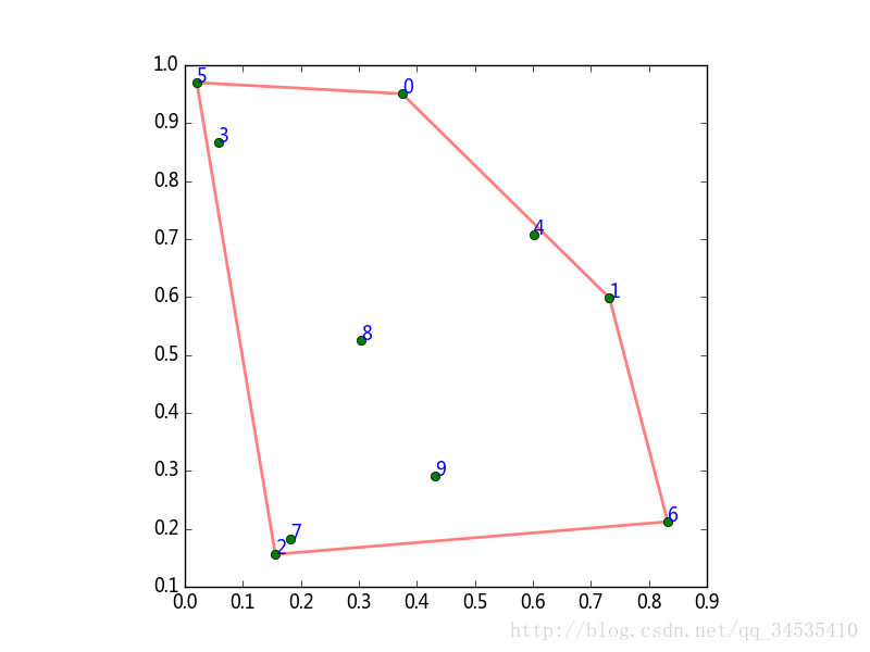


 289
289


 被折叠的 条评论
为什么被折叠?
被折叠的 条评论
为什么被折叠?
 到【灌水乐园】发言


