Inception-V3论文翻译——中英文对照

文章作者：Tyan
博客：noahsnail.com  |  CSDN  |  简书

声明：作者翻译论文仅为学习，如有侵权请联系作者删除博文，谢谢！

翻译论文汇总：https://github.com/SnailTyan/deep-learning-papers-translation

Rethinking the Inception Architecture for Computer Vision

Abstract

Convolutional networks are at the core of most state-of-the-art computer vision solutions for a wide variety of tasks. Since 2014 very deep convolutional networks started to become mainstream, yielding substantial gains in various benchmarks. Although increased model size and computational cost tend to translate to immediate quality gains for most tasks (as long as enough labeled data is provided for training), computational efficiency and low parameter count are still enabling factors for various use cases such as mobile vision and big-data scenarios. Here we are exploring ways to scale up networks in ways that aim at utilizing the added computation as efficiently as possible by suitably factorized convolutions and aggressive regularization. We benchmark our methods on the ILSVRC 2012 classification challenge validation set demonstrate substantial gains over the state of the art: 21.2% top-1 and 5.6% top-5 error for single frame evaluation using a network with a computational cost of 5 billion multiply-adds per inference and with using less than 25 million parameters. With an ensemble of 4 models and multi-crop evaluation, we report 3.5% top-5 error and 17.3% top-1 error.

对许多任务而言，卷积网络是目前最新的计算机视觉解决方案的核心。从2014年开始，深度卷积网络开始变成主流，在各种基准数据集上都取得了实质性成果。对于大多数任务而言，虽然增加的模型大小和计算成本都趋向于转化为直接的质量收益（只要提供足够的标注数据去训练），但计算效率和低参数计数仍是各种应用场景的限制因素，例如移动视觉和大数据场景。目前，我们正在探索增大网络的方法，目标是通过适当的分解卷积和积极的正则化来尽可能地有效利用增加的计算。我们在ILSVRC 2012分类挑战赛的验证集上评估了我们的方法，结果证明我们的方法超过了目前最先进的方法并取得了实质性收益：对于单一框架评估错误率为：21.2% top-1和5.6% top-5，使用的网络计算代价为每次推断需要进行50亿次乘加运算并使用不到2500万的参数。通过四个模型组合和多次评估，我们报告了3.5% top-5和17.3% top-1的错误率。

1. Introduction

Since the 2012 ImageNet competition [16] winning entry by Krizhevsky et al [9], their network “AlexNet” has been successfully applied to a larger variety of computer vision tasks, for example to object-detection [5], segmentation [12], human pose estimation [22], video classification [8], object tracking [23], and superresolution [3].

从2012年Krizhevsky等人[9]赢得了ImageNet竞赛[16]起，他们的网络“AlexNet”已经成功了应用到了许多计算机视觉任务中，例如目标检测[5]，分割[12]，行人姿势评估[22]，视频分类[8]，目标跟踪[23]和超分辨率[3]。

These successes spurred a new line of research that focused on finding higher performing convolutional neural networks. Starting in 2014, the quality of network architectures significantly improved by utilizing deeper and wider networks. VGGNet [18] and GoogLeNet [20] yielded similarly high performance in the 2014 ILSVRC [16] classification challenge. One interesting observation was that gains in the classification performance tend to transfer to significant quality gains in a wide variety of application domains. This means that architectural improvements in deep convolutional architecture can be utilized for improving performance for most other computer vision tasks that are increasingly reliant on high quality, learned visual features. Also, improvements in the network quality resulted in new application domains for convolutional networks in cases where AlexNet features could not compete with hand engineered, crafted solutions, e.g. proposal generation in detection[4].

这些成功推动了一个新研究领域，这个领域主要专注于寻找更高效运行的卷积神经网络。从2014年开始，通过利用更深更宽的网络，网络架构的质量得到了明显改善。VGGNet[18]和GoogLeNet[20]在2014 ILSVRC [16]分类挑战上取得了类似的高性能。一个有趣的发现是在分类性能上的收益趋向于转换成各种应用领域上的显著质量收益。这意味着深度卷积架构上的架构改进可以用来改善大多数越来越多地依赖于高质量、可学习视觉特征的其它计算机视觉任务的性能。网络质量的改善也导致了卷积网络在新领域的应用，在AlexNet特征不能与手工精心设计的解决方案竞争的情况下，例如，检测时的候选区域生成[4]。

Although VGGNet [18] has the compelling feature of architectural simplicity, this comes at a high cost: evaluating the network requires a lot of computation. On the other hand, the Inception architecture of GoogLeNet [20] was also designed to perform well even under strict constraints on memory and computational budget. For example, GoogleNet employed only 5 million parameters, which represented a 12× reduction with respect to its predecessor AlexNet, which used 60 million parameters. Furthermore, VGGNet employed about 3x more parameters than AlexNet.

尽管VGGNet[18]具有架构简洁的强有力特性，但它的成本很高：评估网络需要大量的计算。另一方面，GoogLeNet[20]的Inception架构也被设计为在内存和计算预算严格限制的情况下也能表现良好。例如，GoogleNet只使用了500万参数，与其前身AlexNet相比减少了12倍，AlexNet使用了6000万参数。此外，VGGNet使用了比AlexNet大约多3倍的参数。

The computational cost of Inception is also much lower than VGGNet or its higher performing successors [6]. This has made it feasible to utilize Inception networks in big-data scenarios[17], [13], where huge amount of data needed to be processed at reasonable cost or scenarios where memory or computational capacity is inherently limited, for example in mobile vision settings. It is certainly possible to mitigate parts of these issues by applying specialized solutions to target memory use [2], [15] or by optimizing the execution of certain operations via computational tricks [10]. However, these methods add extra complexity. Furthermore, these methods could be applied to optimize the Inception architecture as well, widening the efficiency gap again.

Inception的计算成本也远低于VGGNet或其更高性能的后继者[6]。这使得可以在大数据场景中[17]，[13]，在大量数据需要以合理成本处理的情况下或在内存或计算能力固有地受限情况下，利用Inception网络变得可行，例如在移动视觉设定中。通过应用针对内存使用的专门解决方案[2]，[15]或通过计算技巧优化某些操作的执行[10]，可以减轻部分这些问题。但是这些方法增加了额外的复杂性。此外，这些方法也可以应用于优化Inception架构，再次扩大效率差距。

Still, the complexity of the Inception architecture makes it more difficult to make changes to the network. If the architecture is scaled up naively, large parts of the computational gains can be immediately lost. Also, [20] does not provide a clear description about the contributing factors that lead to the various design decisions of the GoogLeNet architecture. This makes it much harder to adapt it to new use-cases while maintaining its efficiency. For example, if it is deemed necessary to increase the capacity of some Inception-style model, the simple transformation of just doubling the number of all filter bank sizes will lead to a 4x increase in both computational cost and number of parameters. This might prove prohibitive or unreasonable in a lot of practical scenarios, especially if the associated gains are modest. In this paper, we start with describing a few general principles and optimization ideas that that proved to be useful for scaling up convolution networks in efficient ways. Although our principles are not limited to Inception-type networks, they are easier to observe in that context as the generic structure of the Inception style building blocks is flexible enough to incorporate those constraints naturally. This is enabled by the generous use of dimensional reduction and parallel structures of the Inception modules which allows for mitigating the impact of structural changes on nearby components. Still, one needs to be cautious about doing so, as some guiding principles should be observed to maintain high quality of the models.

然而，Inception架构的复杂性使得更难以对网络进行更改。如果单纯地放大架构，大部分的计算收益可能会立即丢失。此外，[20]并没有提供关于导致GoogLeNet架构的各种设计决策的贡献因素的明确描述。这使得它更难以在适应新用例的同时保持其效率。例如，如果认为有必要增加一些Inception模型的能力，将滤波器组大小的数量加倍的简单变换将导致计算成本和参数数量增加4倍。这在许多实际情况下可能会被证明是禁止或不合理的，尤其是在相关收益适中的情况下。在本文中，我们从描述一些一般原则和优化思想开始，对于以有效的方式扩展卷积网络来说，这被证实是有用的。虽然我们的原则不局限于Inception类型的网络，但是在这种情况下，它们更容易观察，因为Inception类型构建块的通用结构足够灵活，可以自然地合并这些约束。这通过大量使用降维和Inception模块的并行结构来实现，这允许减轻结构变化对邻近组件的影响。但是，对于这样做需要谨慎，因为应该遵守一些指导原则来保持模型的高质量。

2. General Design Principles

Here we will describe a few design principles based on large-scale experimentation with various architectural choices with convolutional networks. At this point, the utility of the principles below are speculative and additional future experimental evidence will be necessary to assess their accuracy and domain of validity. Still, grave deviations from these principles tended to result in deterioration in the quality of the networks and fixing situations where those deviations were detected resulted in improved architectures in general.

2. 通用设计原则

这里我们将介绍一些具有卷积网络的、具有各种架构选择的、基于大规模实验的设计原则。在这一点上，以下原则的效用是推测性的，另外将来的实验证据将对于评估其准确性和有效领域是必要的。然而，严重偏移这些原则往往会导致网络质量的恶化，修正检测到的这些偏差状况通常会导致改进的架构。

1. Avoid representational bottlenecks, especially early in the network. Feed-forward networks can be represented by an acyclic graph from the input layer(s) to the classifier or regressor. This defines a clear direction for the information flow. For any cut separating the inputs from the outputs, one can access the amount of information passing though the cut. One should avoid bottlenecks with extreme compression. In general the representation size should gently decrease from the inputs to the outputs before reaching the final representation used for the task at hand. Theoretically, information content can not be assessed merely by the dimensionality of the representation as it discards important factors like correlation structure; the dimensionality merely provides a rough estimate of information content.

2. Higher dimensional representations are easier to process locally within a network. Increasing the activations per tile in a convolutional network allows for more disentangled features. The resulting networks will train faster.

3. Spatial aggregation can be done over lower dimensional embeddings without much or any loss in representational power. For example, before performing a more spread out (e.g. 3 × 3) convolution, one can reduce the dimension of the input representation before the spatial aggregation without expecting serious adverse effects. We hypothesize that the reason for that is the strong correlation between adjacent unit results in much less loss of information during dimension reduction, if the outputs are used in a spatial aggregation context. Given that these signals should be easily compressible, the dimension reduction even promotes faster learning.

4. Balance the width and depth of the network. Optimal performance of the network can be reached by balancing the number of filters per stage and the depth of the network. Increasing both the width and the depth of the network can contribute to higher quality networks. However, the optimal improvement for a constant amount of computation can be reached if both are increased in parallel. The computational budget should therefore be distributed in a balanced way between the depth and width of the network.

5. 避免表征瓶颈，尤其是在网络的前面。前馈网络可以由从输入层到分类器或回归器的非循环图表示。这为信息流定义了一个明确的方向。对于分离输入输出的任何切口，可以访问通过切口的信息量。应该避免极端压缩的瓶颈。一般来说，在达到用于着手任务的最终表示之前，表示大小应该从输入到输出缓慢减小。理论上，信息内容不能仅通过表示的维度来评估，因为它丢弃了诸如相关结构的重要因素；维度仅提供信息内容的粗略估计。

6. 更高维度的表示在网络中更容易局部处理。在卷积网络中增加每个图块的激活允许更多解耦的特征。所产生的网络将训练更快。

7. 空间聚合可以在较低维度嵌入上完成，而不会在表示能力上造成许多或任何损失。例如，在执行更多展开（例如3×3）卷积之前，可以在空间聚合之前减小输入表示的维度，没有预期的严重不利影响。我们假设，如果在空间聚合上下文中使用输出，则相邻单元之间的强相关性会导致维度缩减期间的信息损失少得多。鉴于这些信号应该易于压缩，因此尺寸减小甚至会促进更快的学习。

8. 平衡网络的宽度和深度。通过平衡每个阶段的滤波器数量和网络的深度可以达到网络的最佳性能。增加网络的宽度和深度可以有助于更高质量的网络。然而，如果两者并行增加，则可以达到恒定计算量的最佳改进。因此，计算预算应该在网络的深度和宽度之间以平衡方式进行分配。

Although these principles might make sense, it is not straightforward to use them to improve the quality of networks out of box. The idea is to use them judiciously in ambiguous situations only.

虽然这些原则可能是有意义的，但并不是开箱即用的直接使用它们来提高网络质量。我们的想法是仅在不明确的情况下才明智地使用它们。

3. Factorizing Convolutions with Large Filter Size

Much of the original gains of the GoogLeNet network [20] arise from a very generous use of dimension reduction. This can be viewed as a special case of factorizing convolutions in a computationally efficient manner. Consider for example the case of a 1 × 1 convolutional layer followed by a 3 × 3 convolutional layer. In a vision network, it is expected that the outputs of near-by activations are highly correlated. Therefore, we can expect that their activations can be reduced before aggregation and that this should result in similarly expressive local representations.

3. 基于大滤波器尺寸分解卷积

GoogLeNet网络[20]的大部分初始收益来源于大量地使用降维。这可以被视为以计算有效的方式分解卷积的特例。考虑例如1×1卷积层之后接一个3×3卷积层的情况。在视觉网络中，预期相近激活的输出是高度相关的。因此，我们可以预期，它们的激活可以在聚合之前被减少，并且这应该会导致类似的富有表现力的局部表示。

Here we explore other ways of factorizing convolutions in various settings, especially in order to increase the computational efficiency of the solution. Since Inception networks are fully convolutional, each weight corresponds to one multiplication per activation. Therefore, any reduction in computational cost results in reduced number of parameters. This means that with suitable factorization, we can end up with more disentangled parameters and therefore with faster training. Also, we can use the computational and memory savings to increase the filter-bank sizes of our network while maintaining our ability to train each model replica on a single computer.

在这里，我们将在各种设定中探索卷积分解的其它方法，特别是为了提高解决方案的计算效率。由于Inception网络是全卷积的，每个权重对应每个激活的一次乘法。因此，任何计算成本的降低会导致参数数量减少。这意味着，通过适当的分解，我们可以得到更多的解耦参数，从而加快训练。此外，我们可以使用计算和内存节省来增加我们网络的滤波器组的大小，同时保持我们在单个计算机上训练每个模型副本的能力。

3.1. Factorization into smaller convolutions

Convolutions with larger spatial filters (e.g. 5 × 5 or 7 × 7) tend to be disproportionally expensive in terms of computation. For example, a 5 × 5 convolution with n filters over a grid with m filters is 25/9 = 2.78 times more computationally expensive than a 3 × 3 convolution with the same number of filters. Of course, a 5 × 5 filter can capture dependencies between signals between activations of units further away in the earlier layers, so a reduction of the geometric size of the filters comes at a large cost of expressiveness. However, we can ask whether a 5 × 5 convolution could be replaced by a multi-layer network with less parameters with the same input size and output depth. If we zoom into the computation graph of the 5 × 5 convolution, we see that each output looks like a small fully-connected network sliding over 5 × 5 tiles over its input (see Figure 1). Since we are constructing a vision network, it seems natural to exploit translation invariance again and replace the fully connected component by a two layer convolutional architecture: the first layer is a 3 × 3 convolution, the second is a fully connected layer on top of the 3 × 3 output grid of the first layer (see Figure 1). Sliding this small network over the input activation grid boils down to replacing the 5 × 5 convolution with two layers of 3 × 3 convolution (compare Figure 4 with 5).

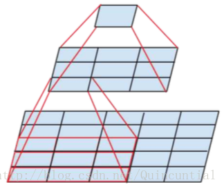
Figure 1. Mini-network replacing the 5×5 convolutions.

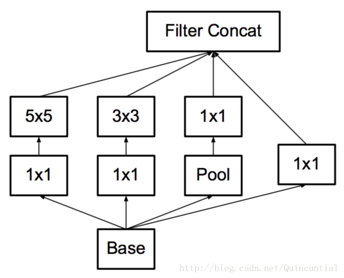
Figure 4. Original Inception module as described in [20].

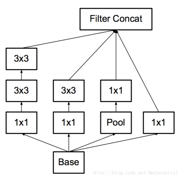
Figure 5. Inception modules where each 5 × 5 convolution is replaced by two 3 × 3 convolution, as suggested by principle 3 of Section 2.

3.1. 分解到更小的卷积

具有较大空间滤波器（例如5×5或7×7）的卷积在计算方面往往不成比例地昂贵。例如，具有n个滤波器的5×5卷积在具有m个滤波器的网格上比具有相同数量的滤波器的3×3卷积的计算量高25/9=2.78倍。当然，5×5滤波器在更前面的层可以捕获更远的单元激活之间、信号之间的依赖关系，因此滤波器几何尺寸的减小带来了很大的表现力。然而，我们可以询问5×5卷积是否可以被具有相同输入尺寸和输出深度的参数较小的多层网络所取代。如果我们放大5×5卷积的计算图，我们看到每个输出看起来像一个小的完全连接的网络，在其输入上滑过5×5的块（见图1）。由于我们正在构建视觉网络，所以通过两层的卷积结构再次利用平移不变性来代替全连接的组件似乎是很自然的：第一层是3×3卷积，第二层是在第一层的3×3输出网格之上的一个全连接层（见图1）。通过在输入激活网格上滑动这个小网络，用两层3×3卷积来替换5×5卷积（比较图4和5）。

图1。Mini网络替换5×5卷积

图4。[20]中描述的最初的Inception模块.

图5。Inception模块中每个5×5卷积由两个3×3卷积替换，正如第2小节中原则3建议的那样。

This setup clearly reduces the parameter count by sharing the weights between adjacent tiles. To analyze the expected computational cost savings, we will make a few simplifying assumptions that apply for the typical situations: We can assume that $n = \alpha m$, that is that we want to change the number of activations/unit by a constant alpha factor. Since the 5 × 5 convolution is aggregating, $\alpha$ is typically slightly larger than one (around 1.5 in the case of GoogLeNet). Having a two layer replacement for the 5 × 5 layer, it seems reasonable to reach this expansion in two steps: increasing the number of filters by $\sqrt \alpha$ in both steps. In order to simplify our estimate by choosing $\alpha = 1$(no expansion), if we would naivly slide a network without reusing the computation between neighboring grid tiles, we would increase the computational cost. Sliding this network can be represented by two 3 × 3 convolutional layers which reuses the activations between adjacent tiles. This way, we end up with a net $\frac {9+9} {25} ×$ reduction of computation, resulting in a relative gain of 28% by this factorization. The exact same saving holds for the parameter count as each parameter is used exactly once in the computation of the activation of each unit. Still, this setup raises two general questions: Does this replacement result in any loss of expressiveness? If our main goal is to factorize the linear part of the computation, would it not suggest to keep linear activations in the first layer? We have ran several control experiments (for example see figure 2) and using linear activation was always inferior to using rectified linear units in all stages of the factorization. We attribute this gain to the enhanced space of variations that the network can learn especially if we batch-normalize [7] the output activations. One can see similar effects when using linear activations for the dimension reduction components.

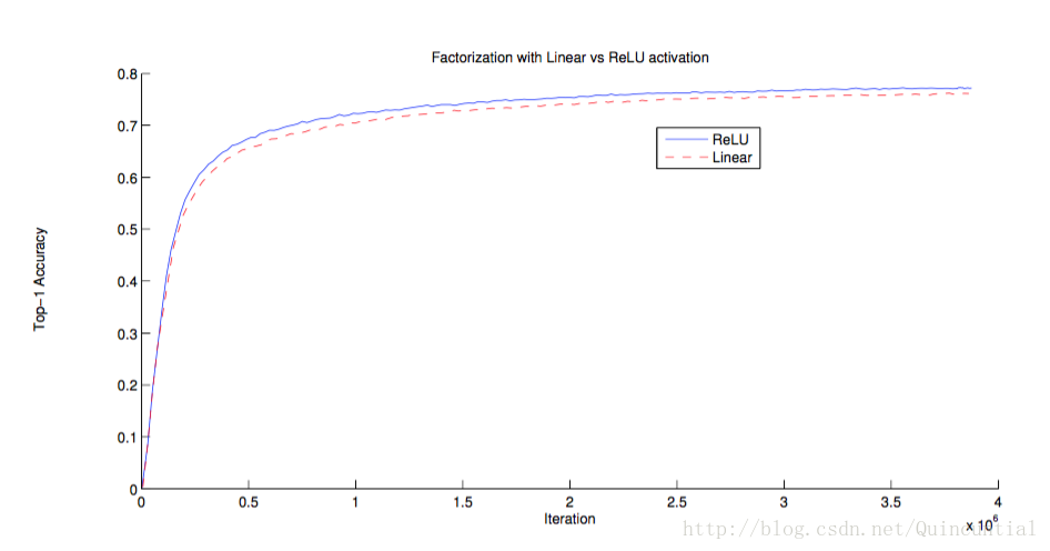
Figure 2. One of several control experiments between two Inception models, one of them uses factorization into linear + ReLU layers, the other uses two ReLU layers. After 3.86 million operations, the former settles at 76.2%, while the latter reaches 77.2% top-1 Accuracy on the validation set.

该设定通过相邻块之间共享权重明显减少了参数数量。为了分析预期的计算成本节省，我们将对典型的情况进行一些简单的假设：我们可以假设$n=\alpha m$，也就是我们想通过常数$\alpha$因子来改变激活/单元的数量。由于5×5卷积是聚合的，$\alpha$通常比1略大（在GoogLeNet中大约是1.5）。用两个层替换5×5层，似乎可以通过两个步骤来实现扩展：在两个步骤中通过$\sqrt \alpha$增加滤波器数量。为了简化我们的估计，通过选择$\alpha=1$（无扩展），如果我们单纯地滑动网络而不重新使用相邻网格图块之间的计算，我们将增加计算成本。滑动该网络可以由两个3×3的卷积层表示，其重用相邻图块之间的激活。这样，我们最终得到一个计算量减少到$\frac {9+9} {25} ×$的网络，通过这种分解导致了28％的相对增益。每个参数在每个单元的激活计算中只使用一次，所以参数计数具有完全相同的节约。不过，这个设置提出了两个一般性的问题：这种替换是否会导致任何表征力的丧失？如果我们的主要目标是对计算的线性部分进行分解，是不是建议在第一层保持线性激活？我们已经进行了几个控制实验（例如参见图2），并且在分解的所有阶段中使用线性激活总是逊于使用修正线性单元。我们将这个收益归因于网络可以学习的增强的空间变化，特别是如果我们对输出激活进行批标准化[7]。当对维度减小组件使用线性激活时，可以看到类似的效果。

图2。两个Inception模型间几个控制实验中的一个，其中一个分解为线性层+ ReLU层，另一个使用两个ReLU层。在三亿八千六百万次运算后，在验证集上前者达到了76.2% top-1准确率，后者达到了77.2% top-1的准确率。

3.2. Spatial Factorization into Asymmetric Convolutions

The above results suggest that convolutions with filters larger 3 × 3 might not be generally useful as they can always be reduced into a sequence of 3 × 3 convolutional layers. Still we can ask the question whether one should factorize them into smaller, for example 2 × 2 convolutions. However, it turns out that one can do even better than 2 × 2 by using asymmetric convolutions, e.g. n × 1. For example using a 3 × 1 convolution followed by a 1 × 3 convolution is equivalent to sliding a two layer network with the same receptive field as in a 3 × 3 convolution (see figure 3). Still the two-layer solution is 33% cheaper for the same number of output filters, if the number of input and output filters is equal. By comparison, factorizing a 3 × 3 convolution into a two 2 × 2 convolution represents only a 11% saving of computation.

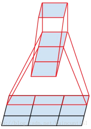
Figure 3. Mini-network replacing the 3 × 3 convolutions. The lower layer of this network consists of a 3 × 1 convolution with 3 output units.

3.2. 空间分解为不对称卷积

上述结果表明，大于3×3的卷积滤波器可能不是通常有用的，因为它们总是可以简化为3×3卷积层序列。我们仍然可以问这个问题，是否应该把它们分解成更小的，例如2×2的卷积。然而，通过使用非对称卷积，可以做出甚至比2×2更好的效果，即n×1。例如使用3×1卷积后接一个1×3卷积，相当于以与3×3卷积相同的感受野滑动两层网络（参见图3）。如果输入和输出滤波器的数量相等，那么对于相同数量的输出滤波器，两层解决方案便宜33％。相比之下，将3×3卷积分解为两个2×2卷积表示仅节省了11％的计算量。

图3。替换3×3卷积的Mini网络。网络的更低层由带有3个输出单元的3×1构成。

In theory, we could go even further and argue that one can replace any n × n convolution by a 1 × n convolution followed by a n × 1 convolution and the computational cost saving increases dramatically as n grows (see figure 6). In practice, we have found that employing this factorization does not work well on early layers, but it gives very good results on medium grid-sizes (On m × m feature maps, where m ranges between 12 and 20). On that level, very good results can be achieved by using 1 × 7 convolutions followed by 7 × 1 convolutions.

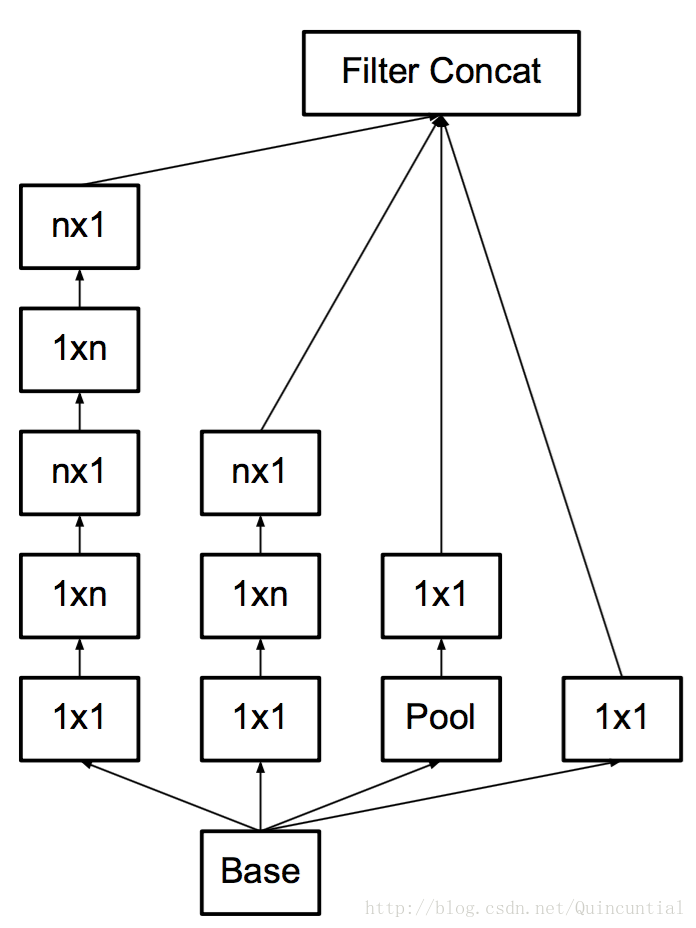
Figure 6. Inception modules after the factorization of the n × n convolutions. In our proposed architecture, we chose n = 7 for the 17 × 17 grid. (The filter sizes are picked using principle 3)

在理论上，我们可以进一步论证，可以通过1×n卷积和后面接一个n×1卷积替换任何n×n卷积，并且随着n增长，计算成本节省显著增加（见图6）。实际上，我们发现，采用这种分解在前面的层次上不能很好地工作，但是对于中等网格尺寸（在m×m特征图上，其中m范围在12到20之间），其给出了非常好的结果。在这个水平上，通过使用1×7卷积，然后是7×1卷积可以获得非常好的结果。

图6。n×n卷积分解后的Inception模块。在我们提出的架构中，对17×17的网格我们选择n=7。（滤波器尺寸可以通过原则3选择）

4. Utility of Auxiliary Classifiers

[20] has introduced the notion of auxiliary classifiers to improve the convergence of very deep networks. The original motivation was to push useful gradients to the lower layers to make them immediately useful and improve the convergence during training by combating the vanishing gradient problem in very deep networks. Also Lee et al[11] argues that auxiliary classifiers promote more stable learning and better convergence. Interestingly, we found that auxiliary classifiers did not result in improved convergence early in the training: the training progression of network with and without side head looks virtually identical before both models reach high accuracy. Near the end of training, the network with the auxiliary branches starts to overtake the accuracy of the network without any auxiliary branch and reaches a slightly higher plateau.

4. 利用辅助分类器

[20]引入了辅助分类器的概念，以改善非常深的网络的收敛。最初的动机是将有用的梯度推向较低层，使其立即有用，并通过抵抗非常深的网络中的消失梯度问题来提高训练过程中的收敛。Lee等人[11]也认为辅助分类器促进了更稳定的学习和更好的收敛。有趣的是，我们发现辅助分类器在训练早期并没有导致改善收敛：在两个模型达到高精度之前，有无侧边网络的训练进度看起来几乎相同。接近训练结束，辅助分支网络开始超越没有任何分支的网络的准确性，达到了更高的稳定水平。

Also [20] used two side-heads at different stages in the network. The removal of the lower auxiliary branch did not have any adverse effect on the final quality of the network. Together with the earlier observation in the previous paragraph, this means that original the hypothesis of [20] that these branches help evolving the low-level features is most likely misplaced. Instead, we argue that the auxiliary classifiers act as regularizer. This is supported by the fact that the main classifier of the network performs better if the side branch is batch-normalized [7] or has a dropout layer. This also gives a weak supporting evidence for the conjecture that batch normalization acts as a regularizer.

另外，[20]在网络的不同阶段使用了两个侧分支。移除更下面的辅助分支对网络的最终质量没有任何不利影响。再加上前一段的观察结果，这意味着[20]最初的假设，这些分支有助于演变低级特征很可能是不适当的。相反，我们认为辅助分类器起着正则化项的作用。这是由于如果侧分支是批标准化的[7]或具有丢弃层，则网络的主分类器性能更好。这也为推测批标准化作为正则化项给出了一个弱支持证据。

5. Efficient Grid Size Reduction

Traditionally, convolutional networks used some pooling operation to decrease the grid size of the feature maps. In order to avoid a representational bottleneck, before applying maximum or average pooling the activation dimension of the network filters is expanded. For example, starting a $d\times d$ grid with $k$ filters, if we would like to arrive at a $\frac{d}{2}\times \frac{d}{2}$ grid with $2k$ filters, we first need to compute a stride-1 convolution with $2k$ filters and then apply an additional pooling step. This means that the overall computational cost is dominated by the expensive convolution on the larger grid using $2d^2k^2$ operations. One possibility would be to switch to pooling with convolution and therefore resulting in $2(\frac{d}{2})^2k^2$ reducing the computational cost by a quarter. However, this creates a representational bottlenecks as the overall dimensionality of the representation drops to $(\frac{d}{2})^2k$ resulting in less expressive networks (see Figure 9). Instead of doing so, we suggest another variant the reduces the computational cost even further while removing the representational bottleneck. (see Figure 10). We can use two parallel stride 2 blocks: $P$ and $C$. $P$ is a pooling layer (either average or maximum pooling) the activation, both of them are stride $2$ the filter banks of which are concatenated as in figure 10.

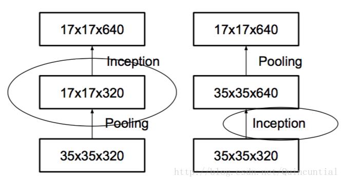
Figure 9. Two alternative ways of reducing the grid size. The solution on the left violates the principle 1 of not introducing an representational bottleneck from Section 2. The version on the right is 3 times more expensive computationally.

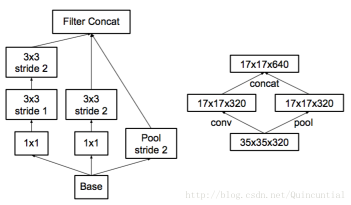
Figure 10. Inception module that reduces the grid-size while expands the filter banks. It is both cheap and avoids the representational bottleneck as is suggested by principle 1. The diagram on the right represents the same solution but from the perspective of grid sizes rather than the operations.

5. 有效的网格尺寸减少

传统上，卷积网络使用一些池化操作来缩减特征图的网格大小。为了避免表示瓶颈，在应用最大池化或平均池化之前，需要扩展网络滤波器的激活维度。例如，开始有一个带有$k$个滤波器的$d \times d$网格，如果我们想要达到一个带有$2k$个滤波器的$\frac{d}{2}\times \frac{d}{2}$网格，我们首先需要用$2k$个滤波器计算步长为1的卷积，然后应用一个额外的池化步骤。这意味着总体计算成本由在较大的网格上使用$2d^2k^2$次运算的昂贵卷积支配。一种可能性是转换为带有卷积的池化，因此导致$2(\frac{d}{2})^2k^2$次运算，将计算成本降低为原来的四分之一。然而，由于表示的整体维度下降到$(\frac{d}{2})^2k$，会导致表示能力较弱的网络（参见图9），这会产生一个表示瓶颈。我们建议另一种变体，其甚至进一步降低了计算成本，同时消除了表示瓶颈（见图10），而不是这样做。我们可以使用两个平行的步长为2的块：$P$和$C$。$P$是一个池化层（平均池化或最大池化）的激活，两者都是步长为$2$，其滤波器组连接如图10所示。

图9。减少网格尺寸的两种替代方式。左边的解决方案违反了第2节中不引入表示瓶颈的原则1。右边的版本计算量昂贵3倍。

图10。缩减网格尺寸的同时扩展滤波器组的Inception模块。它不仅廉价并且避免了原则1中提出的表示瓶颈。右侧的图表示相同的解决方案，但是从网格大小而不是运算的角度来看。

6. Inception-v2

Here we are connecting the dots from above and propose a new architecture with improved performance on the ILSVRC 2012 classification benchmark. The layout of our network is given in table 1. Note that we have factorized the traditional $7\times 7$ convolution into three $3\times 3$ convolutions based on the same ideas as described in section 3.1. For the Inception part of the network, we have $3$ traditional inception modules at the $35\times 35$ with $288$ filters each. This is reduced to a $17 \times 17$ grid with $768$ filters using the grid reduction technique described in section 5. This is is followed by $5$ instances of the factorized inception modules as depicted in figure 5. This is reduced to a $8 \times 8 \times 1280$ grid with the grid reduction technique depicted in figure 10. At the coarsest $8 \times 8$ level, we have two Inception modules as depicted in figure 6, with a concatenated output filter bank size of 2048 for each tile. The detailed structure of the network, including the sizes of filter banks inside the Inception modules, is given in the supplementary material, given in the model.txt that is in the tar-file of this submission. However, we have observed that the quality of the network is relatively stable to variations as long as the principles from Section 2 are observed. Although our network is $42$ layers deep, our computation cost is only about $2.5$ higher than that of GoogLeNet and it is still much more efficient than VGGNet.

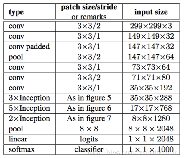
Table 1. The outline of the proposed network architecture. The output size of each module is the input size of the next one. We are using variations of reduction technique depicted Figure 10 to reduce the grid sizes between the Inception blocks whenever applicable. We have marked the convolution with 0-padding, which is used to maintain the grid size. 0-padding is also used inside those Inception modules that do not reduce the grid size. All other layers do not use padding. The various filter bank sizes are chosen to observe principle 4 from Section 2.

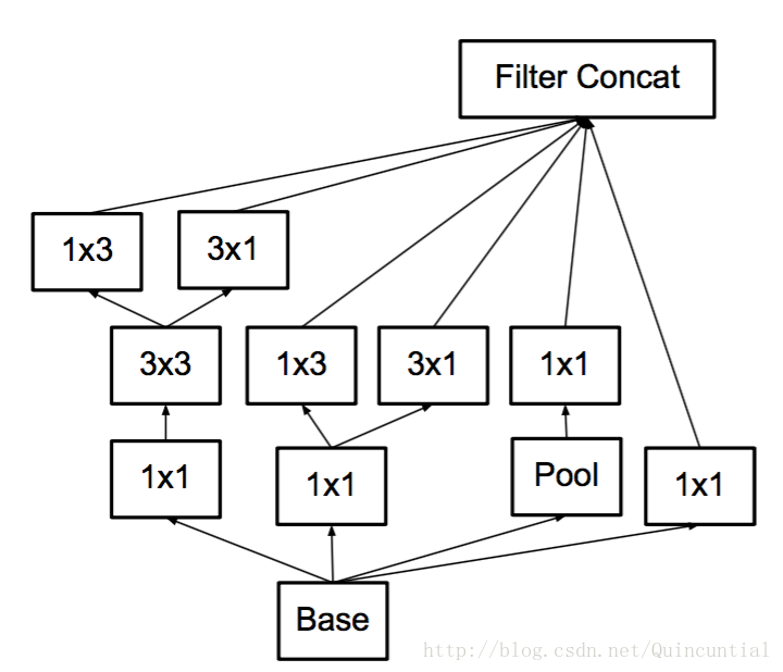
Figure 7. Inception modules with expanded the filter bank outputs. This architecture is used on the coarsest ($8 \times 8$) grids to promote high dimensional representations, as suggested by principle 2 of Section 2. We are using this solution only on the coarsest grid, since that is the place where producing high dimensional sparse representation is the most critical as the ratio of local processing (by $1 \times 1$ convolutions) is increased compared to the spatial aggregation.

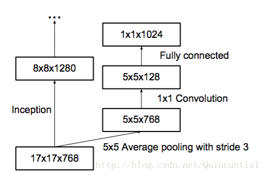
Figure 8. Auxiliary classifier on top of the last $17 \times 17$ layer. Batch normalization[7] of the layers in the side head results in a 0.4% absolute gain in top-1 accuracy. The lower axis shows the number of itertions performed, each with batch size 32.

6. Inception-v2

在这里，我们连接上面的点，并提出了一个新的架构，在ILSVRC 2012分类基准数据集上提高了性能。我们的网络布局在表1中给出。注意，基于与3.1节中描述的同样想法，我们将传统的$7 \times 7$卷积分解为3个$3\times 3$卷积。对于网络的Inception部分，我们在$35 \times 35$处有$3$个传统的Inception模块，每个模块有$288$个滤波器。使用第5节中描述的网格缩减技术，这将缩减为$17\times 17$的网格，具有$768$个滤波器。这之后是图5所示的$5$个分解的Inception模块实例。使用图10所示的网格缩减技术，这被缩减为$8 \times 8 \times 1280$的网格。在最粗糙的$8 \times 8$级别，我们有两个如图6所示的Inception模块，每个块连接的输出滤波器组的大小为2048。网络的详细结构，包括Inception模块内滤波器组的大小，在补充材料中给出，在提交的tar文件中的model.txt中给出。然而，我们已经观察到，只要遵守第2节的原则，对于各种变化网络的质量就相对稳定。虽然我们的网络深度是$42$层，但我们的计算成本仅比GoogLeNet高出约$2.5$倍，它仍比VGGNet要高效的多。

表1。提出的网络架构的轮廓。每个模块的输出大小是下一模块的输入大小。我们正在使用图10所示的缩减技术的变种，以缩减应用时Inception块间的网格大小。我们用0填充标记了卷积，用于保持网格大小。这些Inception模块内部也使用0填充，不会减小网格大小。所有其它层不使用填充。选择各种滤波器组大小来观察第2节的原理4。

图7。具有扩展的滤波器组输出的Inception模块。这种架构被用于最粗糙的（$8 \times 8$）网格，以提升高维表示，如第2节原则2所建议的那样。我们仅在最粗的网格上使用了此解决方案，因为这是产生高维度的地方，稀疏表示是最重要的，因为与空间聚合相比，局部处理（$1 \times 1$ 卷积）的比率增加。

图8。最后$17 \times 17$层之上的辅助分类器。 侧头中的层的批标准化[7]导致top-1 0.4％的绝对收益。下轴显示执行的迭代次数，每个批次大小为32。

7. Model Regularization via Label Smoothing

Here we propose a mechanism to regularize the classifier layer by estimating the marginalized effect of label-dropout during training.

7. 通过标签平滑进行模型正则化

我们提出了一种通过估计训练期间标签丢弃的边缘化效应来对分类器层进行正则化的机制。

For each training example $x$, our model computes the probability of each label $k\in \lbrace 1\ldots K \rbrace$: $p(k|x) = \frac{\exp(z_k)}{\sum_{i=1}^K \exp(z_i)}$. Here, $z_i$ are the logits or unnormalized log-probabilities. Consider the ground-truth distribution over labels $q(k|x)$ for this training example, normalized so that $\sum_k q(k|x) = 1$. For brevity, let us omit the dependence of $p$ and $q$ on example $x$. We define the loss for the example as the cross entropy: $\ell = -\sum_{k=1}^K \log(p(k)) q(k)$. Minimizing this is equivalent to maximizing the expected log-likelihood of a label, where the label is selected according to its ground-truth distribution $q(k)$. Cross-entropy loss is differentiable with respect to the logits $z_k$ and thus can be used for gradient training of deep models. The gradient has a rather simple form: $\frac{\partial\ell}{\partial z_k} = p(k) - q(k)$, which is bounded between $-1$ and $1$.

对于每个训练样本$x$，我们的模型计算每个标签的概率$k\in \lbrace 1\ldots K \rbrace$: $p(k|x) = \frac{\exp(z_k)}{\sum_{i=1}^K \exp(z_i)}$。这里，$z_i$是对数单位或未归一化的对数概率。考虑这个训练样本在标签上的实际分布$q(k|x)$，因此归一化后$\sum_k q(k|x) = 1$。为了简洁，我们省略$p$和$q$对样本$x$的依赖。我们将样本损失定义为交叉熵：$\ell = -\sum_{k=1}^K \log(p(k)) q(k)$。最小化交叉熵等价于最大化标签对数似然期望，其中标签是根据它的实际分布$q(k)$选择的。交叉熵损失对于$z_k$是可微的，因此可以用来进行深度模型的梯度训练。其梯度有一个更简单的形式：$\frac{\partial\ell}{\partial z_k} = p(k) - q(k)$，它的范围在$-1$到$1$之间。

Consider the case of a single ground-truth label $y$, so that $q(y)=1$ and $q(k)=0$ for all $k\neq y$. In this case, minimizing the cross entropy is equivalent to maximizing the log-likelihood of the correct label. For a particular example $x$ with label $y$, the log-likelihood is maximized for $q(k)= \delta_{k,y}$, where $\delta_{k,y}$ is Dirac delta, which equals $1$ for $k=y$ and $0$ otherwise. This maximum is not achievable for finite $z_k$ but is approached if $z_y\gg z_k$ for all $k\neq y$ —— that is, if the logit corresponding to the ground-truth label is much great than all other logits. This, however, can cause two problems. First, it may result in over-fitting: if the model learns to assign full probability to the ground-truth label for each training example, it is not guaranteed to generalize. Second, it encourages the differences between the largest logit and all others to become large, and this, combined with the bounded gradient $\frac{\partial\ell}{\partial z_k}$, reduces the ability of the model to adapt. Intuitively, this happens because the model becomes too confident about its predictions.

考虑单个真实标签$y$的例子，对于所有$k\neq y$，有$q(y)=1$，$q(k)=0$。在这种情况下，最小化交叉熵等价于最大化正确标签的对数似然。对于一个特定的样本$x$，其标签为$y$，对于$q(k)= \delta_{k,y}$，最大化其对数概率，$\delta_{k,y}$为狄拉克δ函数，当且仅当$k=y$时，δ函数值为1，否则为0。对于有限的$z_k$，不能取得最大值，但对于所有$k\neq y$，如果$z_y\gg z_k$——也就是说，如果对应实际标签的逻辑单元远大于其它的逻辑单元，那么对数概率会接近最大值。然而这可能会引起两个问题。首先，它可能导致过拟合：如果模型学习到对于每一个训练样本，分配所有概率到实际标签上，那么它不能保证泛化能力。第二，它鼓励最大的逻辑单元与所有其它逻辑单元之间的差距变大，与有界限的梯度$\frac{\partial\ell}{\partial z_k}$相结合，这会降低模型的适应能力。直观上讲这会发生，因为模型变得对它的预测过于自信。

We propose a mechanism for encouraging the model to be less confident. While this may not be desired if the goal is to maximize the log-likelihood of training labels, it does regularize the model and makes it more adaptable. The method is very simple. Consider a distribution over labels $u(k)$, independent of the training example $x$, and a smoothing parameter $\epsilon$. For a training example with ground-truth label $y$, we replace the label distribution $q(k|x)=\delta_{k,y}$ with

q′(k|x)=(1−ϵ)δk,y+ϵu(k) q ′ ( k | x ) = ( 1 − ϵ ) δ k , y + ϵ u ( k )

$$q'(k|x) = (1-\epsilon) \delta_{k,y} + \epsilon u(k)$$ which is a mixture of the original ground-truth distribution $q(k|x)$ and the fixed distribution $u(k)$, with weights $1-\epsilon$ and $\epsilon$, respectively. This can be seen as the distribution of the label $k$ obtained as follows: first, set it to the ground-truth label $k=y$; then, with probability $\epsilon$, replace $k$ with a sample drawn from the distribution $u(k)$. We propose to use the prior distribution over labels as $u(k)$. In our experiments, we used the uniform distribution $u(k) = 1/K$, so that $$q'(k) = (1-\epsilon) \delta_{k,y} + \frac{\epsilon}{K}.$$ We refer to this change in ground-truth label distribution as label-smoothing regularization, or LSR.

我们提出了一个鼓励模型不那么自信的机制。如果目标是最大化训练标签的对数似然，这可能不是想要的，但它确实使模型正规化并使其更具适应性。这个方法很简单。考虑标签$u(k)$的分布和平滑参数$\epsilon$，与训练样本$x$相互独立。对于一个真实标签为$y$的训练样本，我们用

q′(k|x)=(1−ϵ)δk,y+ϵu(k) q ′ ( k | x ) = ( 1 − ϵ ) δ k , y + ϵ u ( k )

$$q'(k|x) = (1-\epsilon) \delta_{k,y} + \epsilon u(k)$$ 代替标签分布$q(k|x)=\delta_{k,y}$，其由最初的实际分布$q(k|x)$和固定分布$u(k)$混合得到，它们的权重分别为$1-\epsilon$和$\epsilon$。这可以看作获得标签$k$的分布如下：首先，将其设置为真实标签$k=y$；其次，用分布$u(k)$中的采样和概率$\epsilon$替代$k$。我们建议使用标签上的先验分布作为$u(k)$。在我们的实验中，我们使用了均匀分布$u(k) = 1/K$，以便使得 $$q'(k) = (1-\epsilon) \delta_{k,y} + \frac{\epsilon}{K}.$$ 我们将真实标签分布中的这种变化称为标签平滑正则化，或LSR。

Note that LSR achieves the desired goal of preventing the largest logit from becoming much larger than all others. Indeed, if this were to happen, then a single $q(k)$ would approach $1$ while all others would approach $0$. This would result in a large cross-entropy with $q'(k)$ because, unlike $q(k)=\delta_{k,y}$, all $q'(k)$ have a positive lower bound.

注意，LSR实现了期望的目标，阻止了最大的逻辑单元变得比其它的逻辑单元更大。实际上，如果发生这种情况，则一个$q(k)$将接近$1$，而所有其它的将会接近$0$。这会导致$q'(k)$有一个大的交叉熵，因为不同于$q(k)=\delta_{k,y}$，所有的$q'(k)$都有一个正的下界。

Another interpretation of LSR can be obtained by considering the cross entropy:

$$H(q',p) = -\sum_{k=1}^K \log p(k) q'(k) = (1-\epsilon)H(q, p) + \epsilon H(u, p)$$ Thus, LSR is equivalent to replacing a single cross-entropy loss $H(q,p)$ with a pair of such losses $H(q,p)$ and $H(u,p)$. The second loss penalizes the deviation of predicted label distribution $p$ from the prior $u$, with the relative weight $\frac{\epsilon}{1-\epsilon}$. Note that this deviation could be equivalently captured by the KL divergence, since $H(u,p) = D_{KL}(u\|p) + H(u)$ and $H(u)$ is fixed. When $u$ is the uniform distribution, $H(u,p)$ is a measure of how dissimilar the predicted distribution $p$ is to uniform, which could also be measured (but not equivalently) by negative entropy $-H(p)$; we have not experimented with this approach.

LSR的另一种解释可以通过考虑交叉熵来获得：

$$H(q',p) = -\sum_{k=1}^K \log p(k) q'(k) = (1-\epsilon)H(q, p) + \epsilon H(u, p)$$ 因此，LSR等价于用一对这样的损失$H(q,p)$和$H(u,p)$来替换单个交叉熵损失$H(q,p)$。第二个损失惩罚预测的标签分布$p$与先验$u$之间的偏差，其中相对权重为$\frac{\epsilon}{1-\epsilon}$。注意，由于$H(u,p) = D_{KL}(u\|p) + H(u)$和$H(u)$是固定的，因此这个偏差可以等价地被KL散度捕获。当$u$是均匀分布时，$H(u,p)$是度量预测分布$p$与均匀分布不同的程度，也可以通过负熵$-H(p)$来度量（但不等价）；我们还没有实验过这种方法。

In our ImageNet experiments with $K=1000$ classes, we used $u(k) = 1/1000$ and $\epsilon=0.1$. For ILSVRC 2012, we have found a consistent improvement of about $0.2\%$ absolute both for top-$1$ error and the top-$5$ error (cf. Table 3).

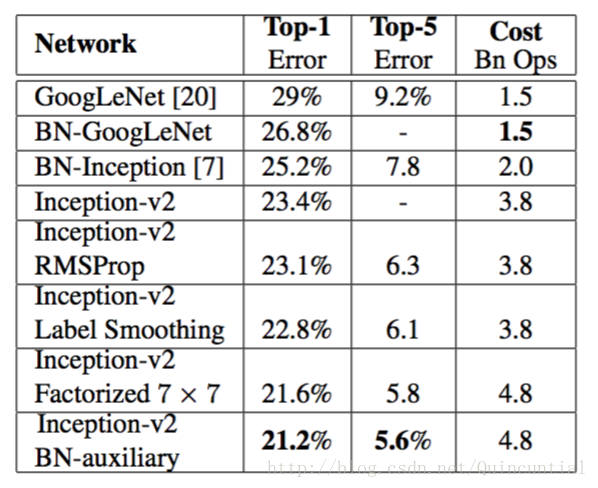
Table 3. Single crop experimental results comparing the cumulative effects on the various contributing factors. We compare our numbers with the best published single-crop inference for Ioffe at al [7]. For the “Inception-v2” lines, the changes are cumulative and each subsequent line includes the new change in addition to the previous ones. The last line is referring to all the changes is what we refer to as “Inception-v3” below. Unfortunately, He et al [6] reports the only 10-crop evaluation results, but not single crop results, which is reported in the Table 4 below.

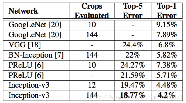
Table 4. Single-model, multi-crop experimental results comparing the cumulative effects on the various contributing factors. We compare our numbers with the best published single-model inference results on the ILSVRC 2012 classification benchmark.

在我们的$K=1000$类的ImageNet实验中，我们使用了$u(k) = 1/1000$和$\epsilon=0.1$。对于ILSVRC 2012，我们发现对于top-1错误率和top-5错误率，持续提高了大约$0.2\%$（参见表3）。

表3。单张裁剪图像的实验结果，比较各种影响因素的累积影响。我们将我们的数据与Ioffe等人[7]发布的单张裁剪图像的最好推断结果进行了比较。在“Inception-v2”行，变化是累积的并且接下来的每一行都包含除了前面的变化之外的新变化。最后一行是所有的变化，我们称为“Inception-v3”。遗憾的是，He等人[6]仅报告了10个裁剪图像的评估结果，但没有单张裁剪图像的结果，报告在下面的表4中。

表4。单模型，多裁剪图像的实验结果，比较各种影响因素的累积影响。我们将我们的数据与ILSVRC 2012分类基准中发布的最佳单模型推断结果进行了比较。

8. Training Methodology

We have trained our networks with stochastic gradient utilizing the TensorFlow [1] distributed machine learning system using $50$ replicas running each on a NVidia Kepler GPU with batch size $32$ for $100$ epochs. Our earlier experiments used momentum [19] with a decay of $0.9$, while our best models were achieved using RMSProp [21] with decay of $0.9$ and $\epsilon=1.0$. We used a learning rate of $0.045$, decayed every two epoch using an exponential rate of $0.94$. In addition, gradient clipping [14] with threshold $2.0$ was found to be useful to stabilize the training. Model evaluations are performed using a running average of the parameters computed over time.

8. 训练方法

我们在TensorFlow[1]分布式机器学习系统上使用随机梯度方法训练了我们的网络，使用了$50$个副本，每个副本在一个NVidia Kepler GPU上运行，批处理大小为$32$，$100$个epoch。我们之前的实验使用动量方法[19]，衰减值为$0.9$，而我们最好的模型是用RMSProp [21]实现的，衰减值为$0.9$，$\epsilon=1.0$。我们使用$0.045$的学习率，每两个epoch以$0.94$的指数速率衰减。此外，阈值为$2.0$的梯度裁剪[14]被发现对于稳定训练是有用的。使用随时间计算的运行参数的平均值来执行模型评估。

9. Performance on Lower Resolution Input

A typical use-case of vision networks is for the the post-classification of detection, for example in the Multibox [4] context. This includes the analysis of a relative small patch of the image containing a single object with some context. The tasks is to decide whether the center part of the patch corresponds to some object and determine the class of the object if it does. The challenge is that objects tend to be relatively small and low-resolution. This raises the question of how to properly deal with lower resolution input.

9. 低分辨率输入上的性能

视觉网络的典型用例是用于检测的后期分类，例如在Multibox [4]上下文中。这包括分析在某个上下文中包含单个对象的相对较小的图像块。任务是确定图像块的中心部分是否对应某个对象，如果是，则确定该对象的类别。这个挑战的是对象往往比较小，分辨率低。这就提出了如何正确处理低分辨率输入的问题。

The common wisdom is that models employing higher resolution receptive fields tend to result in significantly improved recognition performance. However it is important to distinguish between the effect of the increased resolution of the first layer receptive field and the effects of larger model capacitance and computation. If we just change the resolution of the input without further adjustment to the model, then we end up using computationally much cheaper models to solve more difficult tasks. Of course, it is natural, that these solutions loose out already because of the reduced computational effort. In order to make an accurate assessment, the model needs to analyze vague hints in order to be able to “hallucinate” the fine details. This is computationally costly. The question remains therefore: how much does higher input resolution helps if the computational effort is kept constant. One simple way to ensure constant effort is to reduce the strides of the first two layer in the case of lower resolution input, or by simply removing the first pooling layer of the network.

普遍的看法是，使用更高分辨率感受野的模型倾向于导致显著改进的识别性能。然而，区分第一层感受野分辨率增加的效果和较大的模型容量、计算量的效果是很重要的。如果我们只是改变输入的分辨率而不进一步调整模型，那么我们最终将使用计算上更便宜的模型来解决更困难的任务。当然，由于减少了计算量，这些解决方案很自然就出来了。为了做出准确的评估，模型需要分析模糊的提示，以便能够“幻化”细节。这在计算上是昂贵的。因此问题依然存在：如果计算量保持不变，更高的输入分辨率会有多少帮助。确保不断努力的一个简单方法是在较低分辨率输入的情况下减少前两层的步长，或者简单地移除网络的第一个池化层。

For this purpose we have performed the following three experiments:
1. $299\times 299$ receptive field with stride $2$ and maximum pooling after the first layer.
2. $151\times 151$ receptive field with stride $1$ and maximum pooling after the first layer.
3. $79\times 79$ receptive field with stride $1$ and without pooling after the first layer.

All three networks have almost identical computational cost. Although the third network is slightly cheaper, the cost of the pooling layer is marginal and (within $1\%$ of the total cost of the network). In each case, the networks were trained until convergence and their quality was measured on the validation set of the ImageNet ILSVRC 2012 classification benchmark. The results can be seen in table 2. Although the lower-resolution networks take longer to train, the quality of the final result is quite close to that of their higher resolution counterparts.

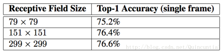
Table 2. Comparison of recognition performance when the size of the receptive field varies, but the computational cost is constant.

为了这个目的我们进行了以下三个实验：
1. 步长为$2$，大小为$299\times 299$的感受野和最大池化。
2. 步长为$1$，大小为$151\times 151$的感受野和最大池化。
3. 步长为$1$，大小为$79\times 79$的感受野和第一层之后没有池化。

所有三个网络具有几乎相同的计算成本。虽然第三个网络稍微便宜一些，但是池化层的成本是无足轻重的（在总成本的$1\%$以内）。在每种情况下，网络都进行了训练，直到收敛，并在ImageNet ILSVRC 2012分类基准数据集的验证集上衡量其质量。结果如表2所示。虽然分辨率较低的网络需要更长时间去训练，但最终结果却与较高分辨率网络的质量相当接近。

表2。当感受野尺寸变化时，识别性能的比较，但计算代价是不变的。

However, if one would just naively reduce the network size according to the input resolution, then network would perform much more poorly. However this would an unfair comparison as we would are comparing a 16 times cheaper model on a more difficult task.

但是，如果只是单纯地按照输入分辨率减少网络尺寸，那么网络的性能就会差得多。然而，这将是一个不公平的比较，因为我们将在比较困难的任务上比较一个便宜16倍的模型。

Also these results of table 2 suggest, one might consider using dedicated high-cost low resolution networks for smaller objects in the R-CNN [5] context.

表2的这些结果也表明，有人可能会考虑在R-CNN [5]的上下文中对更小的对象使用专用的高成本低分辨率网络。

10. Experimental Results and Comparisons

Table 3 shows the experimental results about the recognition performance of our proposed architecture (Inception-v2) as described in Section 6. Each Inception-v2 line shows the result of the cumulative changes including the highlighted new modification plus all the earlier ones. Label Smoothing refers to method described in Section 7. Factorized $7\times 7$ includes a change that factorizes the first $7\times 7$ convolutional layer into a sequence of $3\times 3$ convolutional layers. BN-auxiliary refers to the version in which the fully connected layer of the auxiliary classifier is also batch-normalized, not just the convolutions. We are referring to the model in last row of Table 3 as Inception-v3 and evaluate its performance in the multi-crop and ensemble settings.

10. 实验结果和比较

表3显示了我们提出的体系结构（Inception-v2）识别性能的实验结果，架构如第6节所述。每个Inception-v2行显示了累积变化的结果，包括突出显示的新修改加上所有先前修改的结果。标签平滑是指在第7节中描述的方法。分解的$7\times 7$包括将第一个$7\times 7$卷积层分解成$3\times 3$卷积层序列的改变。BN-auxiliary是指辅助分类器的全连接层也批标准化的版本，而不仅仅是卷积。我们将表3最后一行的模型称为Inception-v3，并在多裁剪图像和组合设置中评估其性能。

All our evaluations are done on the 48238 non-blacklisted examples on the ILSVRC-2012 validation set, as suggested by [16]. We have evaluated all the 50000 examples as well and the results were roughly $0.1\%$ worse in top-5 error and around $0.2\%$ in top-1 error. In the upcoming version of this paper, we will verify our ensemble result on the test set, but at the time of our last evaluation of BN-Inception in spring [7] indicates that the test and validation set error tends to correlate very well.

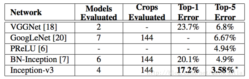
Table 5. Ensemble evaluation results comparing multi-model, multi-crop reported results. Our numbers are compared with the best published ensemble inference results on the ILSVRC 2012 classification benchmark. All results, but the top-5 ensemble result reported are on the validation set. The ensemble yielded 3.46% top-5 error on the validation set.

我们所有的评估都在ILSVRC-2012验证集上的48238个非黑名单样本中完成，如[16]所示。我们也对所有50000个样本进行了评估，结果在top-5错误率中大约为$0.1\%$，在top-1错误率中大约为$0.2\%$。在本文即将出版的版本中，我们将在测试集上验证我们的组合结果，但是我们上一次对BN-Inception的春季测试[7]表明测试集和验证集错误趋于相关性很好。

表5。模型组合评估结果，比较多模型，多裁剪图像的报告结果。我们的数据与ILSVRC 2012分类基准数据集上发布的最好模型组合推断结果的比较。所有的结果，除了在验证集上的top-5模型组合结果。模型组合在验证集上取得了3.46% top-5错误率。

11. Conclusions

We have provided several design principles to scale up convolutional networks and studied them in the context of the Inception architecture. This guidance can lead to high performance vision networks that have a relatively modest computation cost compared to simpler, more monolithic architectures. Our highest quality version of Inception-v3 reaches $21.2\%$, top-$1$ and $5.6\%$ top-5 error for single crop evaluation on the ILSVR 2012 classification, setting a new state of the art. This is achieved with relatively modest ($2.5\times$) increase in computational cost compared to the network described in Ioffe et al [7]. Still our solution uses much less computation than the best published results based on denser networks: our model outperforms the results of He et al [6] —— cutting the top-$5$ (top-$1$) error by $25\%$ ($14\%$) relative, respectively —— while being six times cheaper computationally and using at least five times less parameters (estimated). Our ensemble of four Inception-v3 models reaches $3.5\%$ with multi-crop evaluation reaches $3.5\%$ top-$5$ error which represents an over $25\%$ reduction to the best published results and is almost half of the error of ILSVRC 2014 winining GoogLeNet ensemble.

11. 结论

我们提供了几个设计原则来扩展卷积网络，并在Inception体系结构的背景下进行研究。这个指导可以导致高性能的视觉网络，与更简单、更单一的体系结构相比，它具有相对适中的计算成本。Inception-v3的最高质量版本在ILSVR 2012分类上的单裁剪图像评估中达到了$21.2\％$的top-1错误率和$5.6\％$的top-5错误率，达到了新的水平。与Ioffe等[7]中描述的网络相比，这是通过增加相对适中（$2.5/times$）的计算成本来实​​现的。尽管如此，我们的解决方案所使用的计算量比基于更密集网络公布的最佳结果要少得多：我们的模型比He等[6]的结果更好——将top-5(top-1)的错误率相对分别减少了$25\%$ ($14\%$)，然而在计算代价上便宜了六倍，并且使用了至少减少了五倍的参数（估计值）。我们的四个Inception-v3模型的组合效果达到了$3.5\％$，多裁剪图像评估达到了$3.5\％$的top-5的错误率，这相当于比最佳发布的结果减少了$25\％$以上，几乎是ILSVRC 2014的冠军GoogLeNet组合错误率的一半。

We have also demonstrated that high quality results can be reached with receptive field resolution as low as $79\times 79$. This might prove to be helpful in systems for detecting relatively small objects. We have studied how factorizing convolutions and aggressive dimension reductions inside neural network can result in networks with relatively low computational cost while maintaining high quality. The combination of lower parameter count and additional regularization with batch-normalized auxiliary classifiers and label-smoothing allows for training high quality networks on relatively modest sized training sets.

我们还表明，可以通过感受野分辨率为$79\times 79$的感受野取得高质量的结果。这可能证明在检测相对较小物体的系统中是有用的。我们已经研究了在神经网络中如何分解卷积和积极降维可以导致计算成本相对较低的网络，同时保持高质量。较低的参数数量、额外的正则化、批标准化的辅助分类器和标签平滑的组合允许在相对适中大小的训练集上训练高质量的网络。

References

[1] M. Abadi, A. Agarwal, P. Barham, E. Brevdo, Z. Chen, C. Citro, G. S. Corrado, A. Davis, J. Dean, M. Devin, S. Ghemawat, I. Goodfellow, A. Harp, G. Irving, M. Isard, Y. Jia, R. Jozefowicz, L. Kaiser, M. Kudlur, J. Levenberg, D. Mane ́, R. Monga, S. Moore, D. Murray, C. Olah, M. Schuster, J. Shlens, B. Steiner, I. Sutskever, K. Talwar, P. Tucker, V. Vanhoucke, V. Vasudevan, F. Vie ́gas, O. Vinyals, P. Warden, M. Wattenberg, M. Wicke, Y. Yu, and X. Zheng. TensorFlow: Large-scale machine learning on heterogeneous systems, 2015. Software available from tensorflow.org.

[2] W. Chen, J. T. Wilson, S. Tyree, K. Q. Weinberger, and Y. Chen. Compressing neural networks with the hashing trick. In Proceedings of The 32nd International Conference on Machine Learning, 2015.

[3] C. Dong, C. C. Loy, K. He, and X. Tang. Learning a deep convolutional network for image super-resolution. In Computer Vision–ECCV 2014, pages 184–199. Springer, 2014.

[4] D.Erhan,C.Szegedy,A.Toshev,andD.Anguelov.Scalable object detection using deep neural networks. In Computer Vision and Pattern Recognition (CVPR), 2014 IEEE Conference on, pages 2155–2162. IEEE, 2014.

[5] R. Girshick, J. Donahue, T. Darrell, and J. Malik. Rich feature hierarchies for accurate object detection and semantic segmentation. In Proceedings of the IEEE Conference on Computer Vision and Pattern Recognition (CVPR), 2014.

[6] K. He, X. Zhang, S. Ren, and J. Sun. Delving deep into rectifiers: Surpassing human-level performance on imagenet classification. arXiv preprint arXiv:1502.01852, 2015.

[7] S. Ioffe and C. Szegedy. Batch normalization: Accelerating deep network training by reducing internal covariate shift. In Proceedings of The 32nd International Conference on Machine Learning, pages 448–456, 2015.

[8] A.Karpathy,G.Toderici,S.Shetty,T.Leung,R.Sukthankar, and L. Fei-Fei. Large-scale video classification with convolutional neural networks. In Computer Vision and Pattern Recognition (CVPR), 2014 IEEE Conference on, pages 1725–1732. IEEE, 2014.

[9] A. Krizhevsky, I. Sutskever, and G. E. Hinton. Imagenet classification with deep convolutional neural networks. In Advances in neural information processing systems, pages 1097–1105, 2012.

[10] A. Lavin. Fast algorithms for convolutional neural networks. arXiv preprint arXiv:1509.09308, 2015.

[11] C.-Y.Lee,S.Xie,P.Gallagher,Z.Zhang,andZ.Tu.Deeply-supervised nets. arXiv preprint arXiv:1409.5185, 2014.

[12] J. Long, E. Shelhamer, and T. Darrell. Fully convolutional networks for semantic segmentation. In Proceedings of the IEEE Conference on Computer Vision and Pattern Recognition, pages 3431–3440, 2015.

[13] Y. Movshovitz-Attias, Q. Yu, M. C. Stumpe, V. Shet, S. Arnoud, and L. Yatziv. Ontological supervision for fine grained classification of street view storefronts. In Proceedings of the IEEE Conference on Computer Vision and Pattern Recognition, pages 1693–1702, 2015.

[14] R. Pascanu, T. Mikolov, and Y. Bengio. On the difficulty of training recurrent neural networks. arXiv preprint arXiv:1211.5063, 2012.

[15] D. C. Psichogios and L. H. Ungar. Svd-net: an algorithm that automatically selects network structure. IEEE transactions on neural networks/a publication of the IEEE Neural Networks Council, 5(3):513–515, 1993.

[16] O. Russakovsky, J. Deng, H. Su, J. Krause, S. Satheesh, S. Ma, Z. Huang, A. Karpathy, A. Khosla, M. Bernstein, et al. Imagenet large scale visual recognition challenge. 2014.

[17] F. Schroff, D. Kalenichenko, and J. Philbin. Facenet: A unified embedding for face recognition and clustering. arXiv preprint arXiv:1503.03832, 2015.

[18] K. Simonyan and A. Zisserman. Very deep convolutional networks for large-scale image recognition. arXiv preprint arXiv:1409.1556, 2014.

[19] I. Sutskever, J. Martens, G. Dahl, and G. Hinton. On the importance of initialization and momentum in deep learning. In Proceedings of the 30th
International Conference on Machine Learning (ICML-13), volume 28, pages 1139–1147. JMLR Workshop and Conference Proceedings, May 2013.

[20] C. Szegedy, W. Liu, Y. Jia, P. Sermanet, S. Reed, D. Anguelov, D. Erhan, V. Vanhoucke, and A. Rabinovich. Going deeper with convolutions. In Proceedings of the IEEE Conference on Computer Vision and Pattern Recognition, pages 1–9, 2015.

[21] T. Tieleman and G. Hinton. Divide the gradient by a running average of its recent magnitude. COURSERA: Neural Networks for Machine Learning, 4, 2012. Accessed: 2015-11-05.

[22] A. Toshev and C. Szegedy. Deeppose: Human pose estimation via deep neural networks. In Computer Vision and Pattern Recognition (CVPR), 2014 IEEE Conference on, pages 1653–1660. IEEE, 2014.

[23] N. Wang and D.-Y. Yeung. Learning a deep compact image representation for visual tracking. In Advances in Neural Information Processing Systems, pages 809–817, 2013.