【用python实现《统计学习方法》】之感知机（perceptron)

声明：首先非常感谢李航博士和这篇博文的博主。本文的理论部分主要参考李航博士的《统计学习方法》，而代码实现部分则是在上述的博文基础上完成，并新增了对偶形式的感知机的python实现。

感知机（perceptron）是机器学习中最简单的算法之一，容易理解和实现。笔者将使用python实现感知机的算法（重复造轮子），包括感知机的原始形式和对偶形式。

model

感知机的定义：

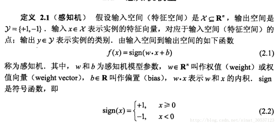
strategy

感知机学习的经验风险函数：

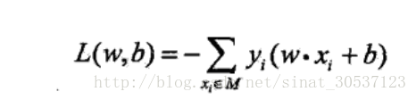
algorithm

原始形式的感知机算法：

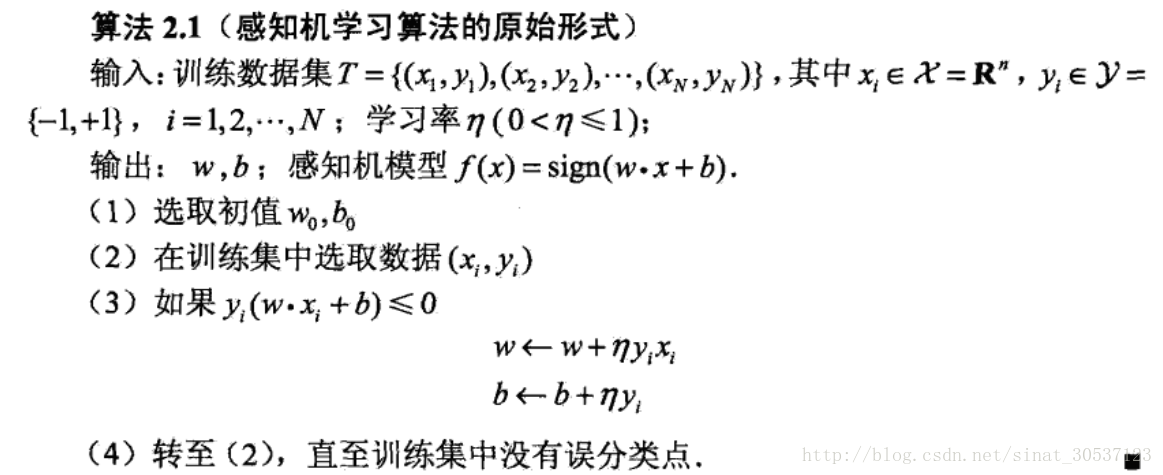
算法的python实现：

import numpy as np
from sklearn.datasets import load_iris
from sklearn.model_selection import train_test_split
import matplotlib.pyplot as plt
from matplotlib.colors import ListedColormap

class Perceptron(object):
    """
    原始形态感知机
    """

    def __init__(self, eta=0.01, n_iter=10):
        self.eta = eta
        self.n_iter = n_iter

    def fit(self, X, y):
        """
        拟合函数，使用训练集来拟合模型
        :param X:training sets
        :param y:training labels
        :return:self
        """
        # X's each col represent a feature
        # initialization wb(weight plus bias)
        self.wb = np.zeros(1 + X.shape[1])
        # the main process of fitting
        self.errors_ = []  # store the errors for each iteration
        for _ in range(self.n_iter):
            errors = 0
            for xi, yi in zip(X, y):
                update = self.eta * (yi - self.predict(xi))
                self.wb[1:] += update * xi
                self.wb[0] += update
                errors += int(update != 0.0)
            self.errors_.append(errors)

        return self

    def net_input(self, xi):
        """
        计算净输入
        :param xi:
        :return:净输入
        """
        return np.dot(xi, self.wb[1:]) + self.wb[0]

    def predict(self, xi):
        """
        计算预测值
        :param xi:
        :return:-1 or 1
        """
        return np.where(self.net_input(xi) <= 0.0, -1, 1)

对偶形式的感知机算法：

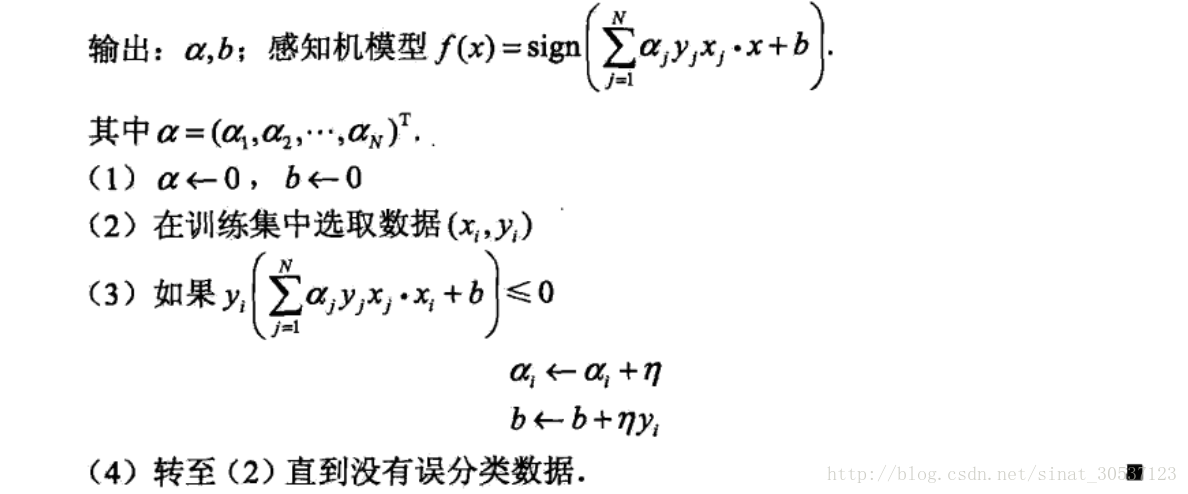
算法的python实现：

a, b, G_matrix = 0, 0, 0

# 计算Gram Matrix
def calculate_g_matrix(data):
    global G_matrix
    G_matrix = np.zeros((data.shape[0], data.shape[0]))
    # 填充Gram Matrix
    for i in range(data.shape[0]):
        for j in range(data.shape[0]):
            G_matrix[i][j] = np.sum(data[i, 0:-1] * data[j, 0:-1])

# 迭代的判定条件
def judge(data, y, index):
    global a, b
    tmp = 0
    for m in range(data.shape[0]):
        tmp += a[m] * data[m, -1] * G_matrix[index][m]

    return (tmp + b) * y


def dual_perceptron(data):
    """
    对偶形态的感知机
    由于对偶形式中训练实例仅以内积的形式出现
    因此，若事先求出Gram Matrix，能大大减少计算量
    :param data:训练数据集;ndarray object
    :return:w,b
    """
    global a, b, G_matrix

    # 计算Gram_Matrix
    calculate_g_matrix(data)

    # 读取数据集中含有的样本数
    num_samples = data.shape[0]
    # 读取数据集中特征向量的个数
    num_features = data.shape[1] - 1
    # 初始化a,b
    a, b = [0] * num_samples, 0
    # 初始化weight
    w = np.zeros((1, num_features))

    i = 0
    while i < num_samples:
        if judge(data, data[i, -1], i) <= 0:
            a[i] += 1
            b += data[i, -1]
            i = 0
        else:
            i += 1

    for j in range(num_samples):
        w += a[j] * data[j, 0:-1] * data[j, -1]

    return w, b

算法实现后需要进行测试，我们先从sklearn.datasets里面获取一个线性可分的数据集iris，并进行交叉验证切割，将数据集分为training set 和test set，最后使用training set 对我们实现的感知机模型进行拟合，代码如下：

def main():
    iris = load_iris()
    X = iris.data[:100, [0, 2]]
    y = iris.target[:100]
    y = np.where(y == 1, 1, -1)
    X_train, X_test, y_train, y_test = \
        train_test_split(X, y, test_size=0.3)
    ppn = Perceptron(eta=0.1, n_iter=10)
    ppn.fit(X_train, y_train)  

然后我们在Perceptron类里面实现一个可视化方法，方法代码如下：

    def plot_decision_regions(self, X, y, resolution=0.02):
        """
        拟合效果可视化
        :param X:training sets
        :param y:training labels
        :param resolution:分辨率
        :return:None
        """
        # initialization colors map
        colors = ['red', 'blue']
        markers = ['o', 'x']
        cmap = ListedColormap(colors[:len(np.unique(y))])

        # plot the decision regions
        x1_max, x1_min = max(X[:, 0]) + 1, min(X[:, 0]) - 1
        x2_max, x2_min = max(X[:, 1]) + 1, min(X[:, 1]) - 1
        xx1, xx2 = np.meshgrid(np.arange(x1_min, x1_max, resolution),
                               np.arange(x2_min, x2_max, resolution))
        Z = self.predict(np.array([xx1.ravel(), xx2.ravel()]).T)
        Z = Z.reshape(xx1.shape)
        plt.contourf(xx1, xx2, Z, alpha=0.4, cmap=cmap)
        plt.xlim(xx1.min(), xx1.max())
        plt.ylim(xx2.min(), xx2.max())

        # plot class samples
        for idx, cl in enumerate(np.unique(y)):
            plt.scatter(x=X[y == cl, 0], y=X[y == cl, 1],
                        alpha=0.8, c=cmap(idx),
                        marker=markers[idx], label=cl)
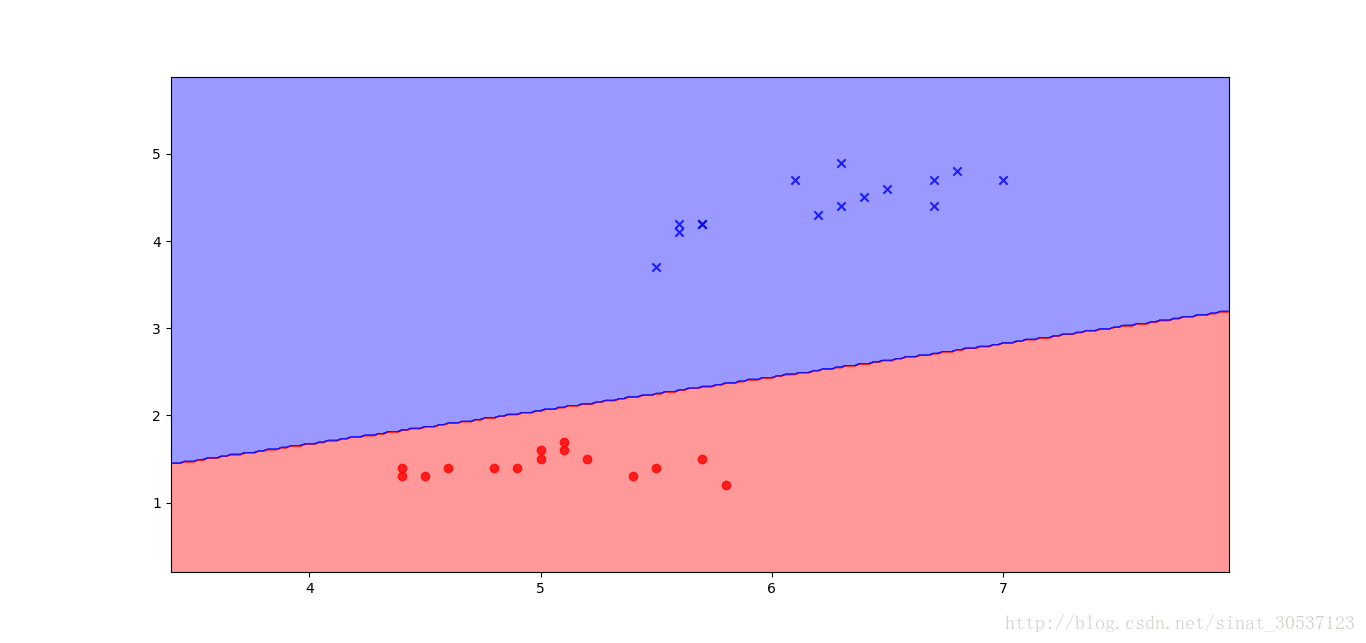
        plt.show()

然后用test set 测试拟合效果：

ppn.plot_decision_regions(X_test, y_test)

效果图如下，可以发现，我们成功的预测出一个模型，能很好的对iris数据集进行分类。

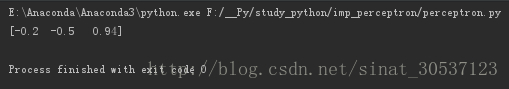
最后，测试一下程序是否正确执行并生成了weight、bias。