指数波段划分以及底部反弹行业特征统计分析

本文参考国金证券杨勇博士最近发的研报《底部反弹特征统计分析》，在优矿网做一个分析实现。

首先是作出指数的波段划分图，用以确定指数的各个底部。

1

import numpy as np

2

import pandas as pd

我写了如下一个函数，可以用于划出各个指数的波段图，虽然写的有点繁琐，但毕竟是可以用。当然我们划出的波段图不仅可以用来找寻顶部、底部。更是可以进一步用来做技术分析，例如波浪理论、缠轮等等。我有关注杨勇老师微信的公众号，其对大盘指数的预测还是非常精准的，用到的也主要是波浪理论、缠轮等。

1

def wave_division(indexid = u"000001.ZICN",begindate = u"20050104", enddate = u"20160530",up_range = 1.2,down_range = 0.85):

2

3

    index = DataAPI.MktIdxdGet(indexID=indexid,beginDate=begindate,endDate=enddate,field=u"tradeDate,lowestIndex,highestIndex",pandas="1")

4

    index = index.set_index(['tradeDate'])

5

    date_flex = [0]

6

    inflexion_flag_high = index.iloc[0]['highestIndex']

7

    inflexion_flag_low = index.iloc[0]['lowestIndex']

8

    m = 0

9

    k = 0

10

    for i in range(len(index)):

11

        #print i,m,k

12

        if i > m  and i > k:

13

            if index.iloc[i]['highestIndex'] / inflexion_flag_low > up_range:

14

                k = i

15

                for j in range(i+1,len(index)):

16

                    #print j,k

17

                    if index.iloc[j]['highestIndex'] > index.iloc[k]['highestIndex']:

18

                        k = j

19

                    elif index.iloc[j]['lowestIndex'] / index.iloc[k]['highestIndex'] < down_range and k != j:

20

                        date_flex.append(k)

21

                        break

22

​

23

            elif index.iloc[i]['lowestIndex'] / inflexion_flag_high < down_range:

24

                m = i

25

                for n in range(i+1,len(index)):

26

                    #print n,m

27

                    if index.iloc[n]['lowestIndex'] < index.iloc[m]['lowestIndex']:

28

                        m = n 

29

                    elif index.iloc[n]['highestIndex'] / index.iloc[m]['lowestIndex'] > up_range and m !=n:

30

                        date_flex.append(m)

31

                        break

32

        else:

33

            pass

34

​

35

        if len(date_flex) > 0:

36

            inflexion_flag_low = index.iloc[max(date_flex)]['lowestIndex']

37

            inflexion_flag_high = index.iloc[max(date_flex)]['highestIndex']

38

39

    #print i,inflexion_flag_low,inflexion_flag_high

40

41

    date_flex.sort()

42

    index['inflexion'] = np.nan

43

44

    if index.iloc[date_flex[1]].mean() > index.iloc[date_flex[0]].mean():

45

        for i in range(len(date_flex)):

46

            if i % 2 == 0:

47

                index['inflexion'].iloc[date_flex[i]] = index.iloc[date_flex[i]]['lowestIndex']

48

            else:

49

                index['inflexion'].iloc[date_flex[i]] = index.iloc[date_flex[i]]['highestIndex']

50

51

    else:

52

        for i in range(len(date_flex)):

53

            if i % 2 == 0:

54

                index['inflexion'].iloc[date_flex[i]] = index.iloc[date_flex[i]]['highestIndex']

55

            else:

56

                index['inflexion'].iloc[date_flex[i]] = index.iloc[date_flex[i]]['lowestIndex']

57

​

58

59

    for i in range(len(index)):

60

        for j in range(len(date_flex)-1):

61

            if i <= date_flex[j+1] and i >= date_flex[j]:

62

                slope = (index['inflexion'].iloc[date_flex[j+1]] - index['inflexion'].iloc[date_flex[j]]) / (date_flex[j+1] - date_flex[j])

63

                index['inflexion'].iloc[i] = slope * (i-date_flex[j]) + index['inflexion'].iloc[date_flex[j]] 

64

65

    return date_flex,index

1

date_flex,cyindex = wave_division(indexid = u"399006.ZICN",begindate = u"20100101", enddate = u"20160530",up_range = 1.1,down_range = 0.92)

1

cyindex.plot(figsize=(20,9),linewidth=2)

1

date_flex,shindex = wave_division()

1

shindex.plot(figsize=(16,9),linewidth=2)

<matplotlib.axes._subplots.AxesSubplot at 0x6252150>

因为波段图就是一个底部一个顶部相交互，我们筛选出底部的时间点与指数低点

1

shindex.iloc[[date_flex[i] for i in range(1,len(date_flex),2)]]

	lowestIndex	highestIndex	inflexion
tradeDate
2005-06-06	998.228	1034.853	998.228
2007-02-06	2541.525	2677.042	2541.525
2007-06-05	3404.146	3768.563	3404.146
2007-07-06	3563.544	3785.346	3563.544
2008-04-22	2990.788	3148.731	2990.788
2008-09-18	1802.331	1942.846	1802.331
2008-10-28	1664.925	1786.435	1664.925
2009-03-03	2037.024	2088.628	2037.024
2009-09-01	2639.759	2727.077	2639.759
2010-07-02	2319.739	2386.400	2319.739
2012-12-04	1949.457	1980.119	1949.457
2013-06-25	1849.653	1963.566	1849.653
2015-07-09	3373.540	3748.479	3373.540
2015-08-26	2850.714	3092.041	2850.714

可以看出与研报中的结果相比，少了2016-01-27这个底部，因为实际上从2016-01-27的2638.3的底部至今没有涨幅超过20%的时候，最多的时候是17%。但没有关系我们还是加上去一起统计。

1

#shindex.iloc[2688].name

2

date_flex.append(2688)

3

shindex.iloc[2688]['inflexion'] = 2638.302

1

shindex.iloc[[date_flex[i] for i in range(1,len(date_flex),2)]]

	lowestIndex	highestIndex	inflexion
tradeDate
2005-06-06	998.228	1034.853	998.228
2007-02-06	2541.525	2677.042	2541.525
2007-06-05	3404.146	3768.563	3404.146
2007-07-06	3563.544	3785.346	3563.544
2008-04-22	2990.788	3148.731	2990.788
2008-09-18	1802.331	1942.846	1802.331
2008-10-28	1664.925	1786.435	1664.925
2009-03-03	2037.024	2088.628	2037.024
2009-09-01	2639.759	2727.077	2639.759
2010-07-02	2319.739	2386.400	2319.739
2012-12-04	1949.457	1980.119	1949.457
2013-06-25	1849.653	1963.566	1849.653
2015-07-09	3373.540	3748.479	3373.540
2015-08-26	2850.714	3092.041	2850.714
2016-01-27	2638.302	2768.772	2638.302

1

bottom_index = shindex.iloc[[date_flex[i] for i in range(1,len(date_flex),2)]]['inflexion']

2

bottom_static = {}

3

for i in range(1,len(date_flex),2):

4

    try:

5

        bottom_static[shindex.iloc[date_flex[i]].name] = [shindex.iloc[date_flex[i+1]]['inflexion'] / shindex.iloc[date_flex[i]]['inflexion'] - 1,date_flex[i+1] - date_flex[i]]

6

    except:

7

        print shindex.iloc[date_flex[i]].name,shindex.iloc[date_flex[i]]['inflexion'],'最后一个底部其反弹多少还不能确定'

2016-01-27

2638.302 最后一个底部其反弹多少还不能确
定

1

bottom_static = pd.DataFrame(bottom_static).T

2

bottom_static = pd.concat([bottom_index,bottom_static],axis=1)

3

bottom_static = bottom_static.rename(columns={'inflexion':'指数低点',0:'反弹幅度',1:'反弹时间长度'})

1

bottom_static

	指数低点	反弹幅度	反弹时间长度
2005-06-06	998.228	1.999597	400
2007-02-06	2541.525	0.706048	70
2007-06-05	3404.146	0.266690	11
2007-07-06	3563.544	0.718526	67
2008-04-22	2990.788	0.265895	8
2008-09-18	1802.331	0.294589	5
2008-10-28	1664.925	0.443192	73
2009-03-03	2037.024	0.707398	106
2009-09-01	2639.759	0.273369	54
2010-07-02	2319.739	0.373741	86
2012-12-04	1949.457	0.254095	46
2013-06-25	1849.653	1.799547	481
2015-07-09	3373.540	0.240373	11
2015-08-26	2850.714	0.292507	78
2016-01-27	2638.302	NaN	NaN

恩，统计的结果和杨勇老师的一模一样呢。接下来我们探索以下底部行业超额收益的情况。

1

from CAL.PyCAL import *

2

import matplotlib.pyplot as plt

3

cal = Calendar('China.SSE')

4

cal.removeHoliday(Date(2007,4,4)) #cal里面的一个小错误，20070404是一个交易日

1

def net_ind_cumret(date_list,indContent):

2

3

    time_list = [[cal.advanceDate(date_list[i], '-20B', BizDayConvention.Unadjusted),cal.advanceDate(date_list[i], '40B', BizDayConvention.Unadjusted)] for i in range(len(for_ind_static))] #得到每个底部日的前20个交易日与后40个交易日

4

5

    #print time_list

6

    #初始化avg_ind_cumret（行业平均累计收益率）

7

    avg_ind_cumret = {}

8

    for ind in indContent.keys():

9

        avg_ind_cumret[ind] = 0

10

11

12

    for i in range(1,len(time_list)): #因为DataAPI.EquRetudGet的数据从06年才开始，故我们不算第一个底部情况，当然也可以使用日线数据直接计算日收益率，此处就不算了

13

14

        index_ret = DataAPI.MktIdxdGet(indexID=u"000001.ZICN",beginDate=time_list[i][0].strftime('%Y%m%d'),endDate=time_list[i][1].strftime('%Y%m%d'),field=['tradeDate','preCloseIndex','closeIndex'],pandas="1")

15

        index_ret['return'] = (index_ret['closeIndex'] - index_ret['preCloseIndex']) / index_ret['preCloseIndex']

16

        #index_cumret = np.array((1 + index_ret['return']).cumprod()) #底部交易日附近指数的累计收益率

17

​

18

        ind_ret = {}

19

        ind_cumret = []

20

21

        for ind in indContent:

22

​

23

            df_ret = DataAPI.EquRetudGet(listStatusCD='L',secID=indContent[ind],beginDate=time_list[i][0].strftime('%Y%m%d'),endDate=time_list[i][1].strftime('%Y%m%d'),field=['secID','tradeDate','dailyReturnReinv'],pandas="1") #得到行业每日收益率

24

            df_marketValue = DataAPI.MktEqudGet(secID=indContent[ind],beginDate=time_list[i][0].strftime('%Y%m%d'),endDate=time_list[i][1].strftime('%Y%m%d'),field=['secID','tradeDate','negMarketValue'],pandas="1")

25

            ##计算行业内指数加权日收益率

26

            df_ret = df_ret.set_index(['tradeDate','secID'])

27

            df_marketValue = df_marketValue.set_index(['tradeDate','secID'])

28

            ind_ret[ind] = (df_ret.unstack() * (df_marketValue.unstack()['negMarketValue'].T / df_marketValue.unstack().sum(axis=1)).T).sum(axis=1) #不想写循环，运用DataFrame的特性

29

            #print ind_ret[ind]

30

31

            for j in range(0,20,5):

32

                ind_cumret.append((1 + ind_ret[ind].iloc[j:20]).prod() - (1 + index_ret['return'].iloc[j:20]).prod())

33

            for j in range(25,61,5):

34

                ind_cumret.append((1 + ind_ret[ind].iloc[20:j]).prod() - (1 + index_ret['return'].iloc[20:j]).prod())

35

36

            avg_ind_cumret[ind] = avg_ind_cumret[ind] + np.array(ind_cumret)

37

38

            ind_cumret = []

39

            #print avg_ind_cumret

40

41

    for key in avg_ind_cumret:

42

        avg_ind_cumret[key] = avg_ind_cumret[key] / (len(time_list) - 1)

43

44

    return avg_ind_cumret

1

def industryGet(tradeDate):             # 设置行业

2

    trade_date = tradeDate

3

    df = DataAPI.EquIndustryGet(industryVersionCD=u"010303",secID = set_universe('HS300',date=trade_date.strftime('%Y%m%d')),intoDate=trade_date.strftime('%Y%m%d'),field=['secID','industryName1','industryName2'])

4

    ind1 = df[df['secID'] == '600000.XSHG']['industryName1'].values[0]

5

    ind2 = df[df['secID'] == '600030.XSHG']['industryName1'].values[0]

6

    industry = df['industryName1'].drop_duplicates().tolist()

7

    if ind1 == ind2 :

8

        industry.remove(ind1)

9

    else:

10

        industry.remove(ind1)

11

        industry.remove(ind2)

12

13

    industry = industry + ['银行','证券','保险','多元金融']

14

    return industry

15

​

16

industry = industryGet(Date(2016,5,26))

17

stkIndustry = DataAPI.EquIndustryGet(industryVersionCD=u"010303",secID = set_universe('A'),intoDate='20160526',field=['secID','industryName1','industryName2'],pandas="1")

18

indContent = {}

19

for ind_name in industry:

20

    indContent[ind_name] = stkIndustry[(stkIndustry['industryName1']==ind_name) | (stkIndustry['industryName2']==ind_name)]['secID'].tolist()

1

avg_ind_cumret = net_ind_cumret(bottom_static[bottom_static['反弹时间长度']>5].index,indContent)

1

index = range(-20,41,5)

2

index.remove(0)

3

avg_ind_cumret = pd.DataFrame(avg_ind_cumret,index=index)

得到底部左右超额收益的相关系数，与研报的结论基本一致，行业超额收益反转的现象，过去超额收益率越高的行业，在底部之后的10个交易日之后将收益率越低。

其中-20表示[-20,0]的超额收益，5表示[0，5]的超额收益

1

avg_ind_cumret.T.corr()

index	-20	-15	-10	-5	5	10	15	20	25	30	35	40
index
-20	1.000000	0.794323	0.735818	0.736515	0.284202	-0.244573	-0.210857	-0.299900	-0.163276	-0.219598	-0.195432	-0.201444
-15	0.794323	1.000000	0.955718	0.821111	0.135788	-0.348093	-0.307521	-0.331221	-0.197013	-0.314560	-0.329344	-0.312431
-10	0.735818	0.955718	1.000000	0.852437	0.020425	-0.463183	-0.430745	-0.435674	-0.308467	-0.425406	-0.414646	-0.404961
-5	0.736515	0.821111	0.852437	1.000000	0.050341	-0.550097	-0.594889	-0.630819	-0.564937	-0.634865	-0.606732	-0.560034
5	0.284202	0.135788	0.020425	0.050341	1.000000	0.543161	0.333631	0.223108	0.147777	0.101948	0.218713	0.233550
10	-0.244573	-0.348093	-0.463183	-0.550097	0.543161	1.000000	0.872429	0.787382	0.667875	0.695969	0.714106	0.719874
15	-0.210857	-0.307521	-0.430745	-0.594889	0.333631	0.872429	1.000000	0.937092	0.883634	0.906957	0.887450	0.890454
20	-0.299900	-0.331221	-0.435674	-0.630819	0.223108	0.787382	0.937092	1.000000	0.917893	0.897338	0.884300	0.875722
25	-0.163276	-0.197013	-0.308467	-0.564937	0.147777	0.667875	0.883634	0.917893	1.000000	0.960722	0.929674	0.902757
30	-0.219598	-0.314560	-0.425406	-0.634865	0.101948	0.695969	0.906957	0.897338	0.960722	1.000000	0.944350	0.912436
35	-0.195432	-0.329344	-0.414646	-0.606732	0.218713	0.714106	0.887450	0.884300	0.929674	0.944350	1.000000	0.982007
40	-0.201444	-0.312431	-0.404961	-0.560034	0.233550	0.719874	0.890454	0.875722	0.902757	0.912436	0.982007	1.000000

1

plt.figure(figsize=(20,15))

2

for x in avg_ind_cumret.columns:

3

    plt.plot(avg_ind_cumret.index, avg_ind_cumret[x])

4

# plt.plot(avg_ind_cumret)

5

plt.legend([e.decode('utf-8') for e in avg_ind_cumret.columns],loc='upper left',prop = font)

<matplotlib.legend.Legend at 0x109946d0>

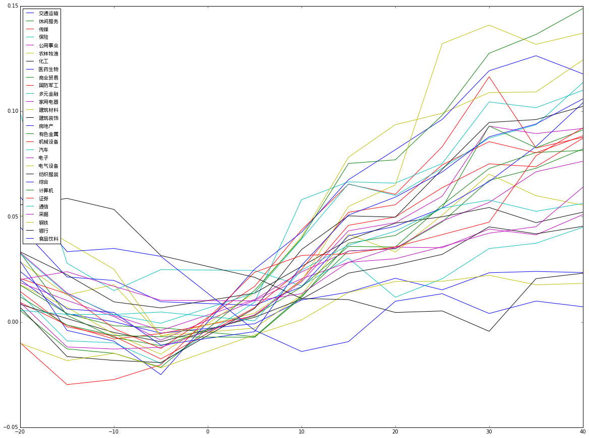
结果与研报的有所不同，可能是行业收益率的计算方式不同，以及我舍去了第一个底部的数据。

我们看下处于反弹时，我们分析结果推荐的行业

1

avg_ind_cumret.ix[5].order(ascending=False).head(5)

房地产 0.025092保险 0.024473证券 0.023604银行 0.021189国防军工 0.016889Name: 5, dtype: float6

4

1

avg_ind_cumret.ix[10].order(ascending=False).head(5)

多元金融 0.058046国防军工 0.043713房地产 0.042585建筑材料 0.040470有色金属 0.039688Name: 10, dtype: float6

4

1

avg_ind_cumret.ix[20].order(ascending=False).head(5)

建筑材料 0.093642房地产 0.081750有色金属 0.076970多元金融 0.065906电气设备 0.065045Name: 20, dtype: float6

4

1

avg_ind_cumret.ix[30].order(ascending=False).head(5)

电气设备 0.140919有色金属 0.127539房地产 0.119225国防军工 0.116397建筑材料 0.108876Name: 30, dtype: float6

4

1

avg_ind_cumret.ix[40].order(ascending=False).head(5)

有色金属 0.148778电气设备 0.137068建筑材料 0.124374房地产 0.117752汽车 0.113629Name: 40, dtype: float6

4

总结一下

反弹的带头大哥都是银行、保险、证券和房地产等行业，但往后走银行等金融行业的收益率在不断下降，而房地产仍能保持不错的收益率。反弹多天后推荐的行业是有色金属、电气设备、建筑材料、汽车等。