机器学习案例实战：信用卡欺诈检测

故事背景

原始数据为个人交易记录，但是考虑数据本身的隐私性，已经对原始数据进行了类似PCA的处理，现在已经把特征数据提取好了，接下来的目的就是如何建立模型使得检测的效果达到最好，这里我们虽然不需要对数据做特征提取的操作，但是面对的挑战还是蛮大的。

import pandas as pd
import matplotlib.pyplot as plt
import numpy as np
from sklearn.cross_validation import train_test_split
from sklearn.linear_model import LogisticRegression
from sklearn.cross_validation import KFold, cross_val_score
from sklearn.metrics import confusion_matrix,recall_score,classification_report 

数据分析与建模可不是体力活，时间就是金钱我的朋友（魔兽玩家都懂的！）如果你用Python来把玩数据，那么这些就是你的核武器啦。简单介绍一下这几位朋友！
Numpy-科学计算库 主要用来做矩阵运算，什么？你不知道哪里会用到矩阵，那么这样想吧，咱们的数据就是行（样本）和列（特征）组成的，那么数据本身不就是一个矩阵嘛。

Pandas-数据分析处理库 很多小伙伴都在说用python处理数据很容易，那么容易在哪呢？其实有了pandas很复杂的操作我们也可以一行代码去解决掉！
Matplotlib-可视化库 无论是分析还是建模，光靠好记性可不行，很有必要把结果和过程可视化的展示出来。

Scikit-Learn-机器学习库 非常实用的机器学习算法库，这里面包含了基本你觉得你能用上所有机器学习算法啦。但还远不止如此，还有很多预处理和评估的模块等你来挖掘的！

data = pd.read_csv("creditcard.csv")
data.head()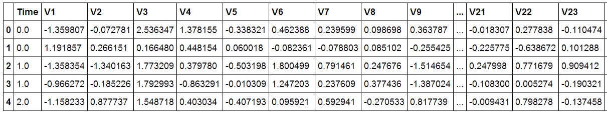

首先我们用pandas将数据读进来并显示最开始的5行，看见木有！用pandas读取数据就是这么简单！这里的数据为了考虑用户隐私等，已经通过PCA处理过了，现在大家只需要把数据当成是处理好的特征就好啦！

接下来我们核心的目的就是去检测在数据样本中哪些是具有欺诈行为的！

count_classes = pd.value_counts(data['Class'], sort = True).sort_index()
count_classes.plot(kind = 'bar')
plt.title("Fraud class histogram")
plt.xlabel("Class")
plt.ylabel("Frequency")

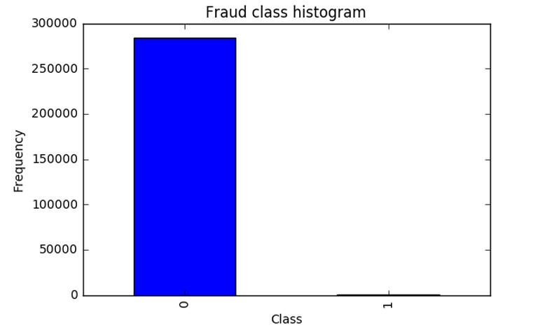
千万不要着急去用机器学习算法建模做这个分类问题。首先我们来观察一下数据的分布情况，在数据样本中有明确的label列指定了class为0代表正常情况，class为1代表发生了欺诈行为的样本。从上图中可以看出来。。。等等，你不是说有两种情况吗，为啥图上只有class为0的样本啊？再仔细看看，纳尼。。。class为1的并不是木有，而是太少了，少到基本看不出来了，那么此时我们面对一个新的挑战，样本极度不均衡，接下来我们首先要解决这个问题，这个很常见也是很头疼的问题。

这里我们提出两种解决方案 也是数据分析中最常用的两种方法，下采样和过采样！

先挑个软柿子捏，下采样比较简单实现，咱们就先搞定第一种方案！下采样的意思就是说，不是两类数据不均衡吗，那我让你们同样少（也就是1有多少个 0就消减成多少个），这样不就均衡了吗?

X = data.ix[:, data.columns != 'Class']
y = data.ix[:, data.columns == 'Class']

# Number of data points in the minority class
number_records_fraud = len(data[data.Class == 1])
fraud_indices = np.array(data[data.Class == 1].index)

# Picking the indices of the normal classes
normal_indices = data[data.Class == 0].index

# Out of the indices we picked, randomly select "x" number (number_records_fraud)
random_normal_indices = np.random.choice(normal_indices, number_records_fraud, replace = False)
random_normal_indices = np.array(random_normal_indices)

# Appending the 2 indices
under_sample_indices = np.concatenate([fraud_indices,random_normal_indices])

# Under sample dataset
under_sample_data = data.iloc[under_sample_indices,:]

X_undersample = under_sample_data.ix[:, under_sample_data.columns != 'Class']
y_undersample = under_sample_data.ix[:, under_sample_data.columns == 'Class']

# Showing ratio
print("Percentage of normal transactions: ", len(under_sample_data[under_sample_data.Class == 0])/len(under_sample_data))
print("Percentage of fraud transactions: ", len(under_sample_data[under_sample_data.Class == 1])/len(under_sample_data))
print("Total number of transactions in resampled data: ", len(under_sample_data))

Percentage of normal transactions:  0.5
Percentage of fraud transactions:  0.5
Total number of transactions in resampled data:  984

很简单的实现方法，在属于0的数据中，进行随机的选择，就选跟class为1的那类样本一样多就好了，那么现在我们已经得到了两组都是非常少的数据，接下来就可以建模啦！不过在建立任何一个机器学习模型之前不要忘了一个常规的操作，就是要把数据集切分成训练集和测试集，这样会使得后续验证的结果更为靠谱。

def printing_Kfold_scores(x_train_data,y_train_data):
    fold = KFold(len(y_train_data),5,shuffle=False) 

    # Different C parameters
    c_param_range = [0.01,0.1,1,10,100]

    results_table = pd.DataFrame(index = range(len(c_param_range),2), columns = ['C_parameter','Mean recall score'])
    results_table['C_parameter'] = c_param_range

    # the k-fold will give 2 lists: train_indices = indices[0], test_indices = indices[1]
    j = 0
    for c_param in c_param_range:
        print('-------------------------------------------')
        print('C parameter: ', c_param)
        print('-------------------------------------------')
        print('')

        recall_accs = []
        for iteration, indices in enumerate(fold,start=1):

            # Call the logistic regression model with a certain C parameter
            lr = LogisticRegression(C = c_param, penalty = 'l1')

            # Use the training data to fit the model. In this case, we use the portion of the fold to train the model
            # with indices[0]. We then predict on the portion assigned as the 'test cross validation' with indices[1]
            lr.fit(x_train_data.iloc[indices[0],:],y_train_data.iloc[indices[0],:].values.ravel())

            # Predict values using the test indices in the training data
            y_pred_undersample = lr.predict(x_train_data.iloc[indices[1],:].values)

            # Calculate the recall score and append it to a list for recall scores representing the current c_parameter
            recall_acc = recall_score(y_train_data.iloc[indices[1],:].values,y_pred_undersample)
            recall_accs.append(recall_acc)
            print('Iteration ', iteration,': recall score = ', recall_acc)

        # The mean value of those recall scores is the metric we want to save and get hold of.
        results_table.ix[j,'Mean recall score'] = np.mean(recall_accs)
        j += 1
        print('')
        print('Mean recall score ', np.mean(recall_accs))
        print('')

    best_c = results_table.loc[results_table['Mean recall score'].idxmax()]['C_parameter']

    # Finally, we can check which C parameter is the best amongst the chosen.
    print('*********************************************************************************')
    print('Best model to choose from cross validation is with C parameter = ', best_c)
    print('*********************************************************************************')

    return best_c
best_c = printing_Kfold_scores(X_train_undersample,y_train_undersample)

上述代码中做了一件非常常规的事情，就是对于一个模型，咱们再选择一个算法的时候伴随着很多的参数要调节，那么如何找到最合适的参数可不是一件简单的事，依靠经验值并不是十分靠谱，通常情况下我们需要大量的实验也就是不断去尝试最终得出这些合适的参数。

不同C参数对应的最终模型效果：

C parameter: 0.01

Iteration 1 : recall score = 0.958904109589
Iteration 2 : recall score = 0.917808219178
Iteration 3 : recall score = 1.0
Iteration 4 : recall score = 0.972972972973
Iteration 5 : recall score = 0.954545454545

Mean recall score 0.960846151257

C parameter: 0.1

Iteration 1 : recall score = 0.835616438356
Iteration 2 : recall score = 0.86301369863
Iteration 3 : recall score = 0.915254237288
Iteration 4 : recall score = 0.932432432432
Iteration 5 : recall score = 0.878787878788

Mean recall score 0.885020937099

C parameter: 1

Iteration 1 : recall score = 0.835616438356
Iteration 2 : recall score = 0.86301369863
Iteration 3 : recall score = 0.966101694915
Iteration 4 : recall score = 0.945945945946
Iteration 5 : recall score = 0.893939393939

Mean recall score 0.900923434357

C parameter: 10

Iteration 1 : recall score = 0.849315068493
Iteration 2 : recall score = 0.86301369863
Iteration 3 : recall score = 0.966101694915
Iteration 4 : recall score = 0.959459459459
Iteration 5 : recall score = 0.893939393939

Mean recall score 0.906365863087

C parameter: 100

Iteration 1 : recall score = 0.86301369863
Iteration 2 : recall score = 0.86301369863
Iteration 3 : recall score = 0.966101694915
Iteration 4 : recall score = 0.959459459459
Iteration 5 : recall score = 0.893939393939

Mean recall score 0.909105589115

Best model to choose from cross validation is with C parameter = 0.01

在使用机器学习算法的时候，很重要的一部就是参数的调节，在这里我们选择使用最经典的分类算法，逻辑回归！千万别把逻辑回归当成是回归算法，它就是最实用的二分类算法！这里我们需要考虑的c参数就是正则化惩罚项的力度，那么如何选择到最好的参数呢？这里我们就需要交叉验证啦，然后用不同的C参数去跑相同的数据，目的就是去看看啥样的C参数能够使得最终模型的效果最好！可以到不同的参数对最终的结果产生的影响还是蛮大的，这里最好的方法就是用验证集去寻找了！

模型已经造出来了，那么怎么评判哪个模型好，哪个模型不好呢？我们这里需要好好想一想！

一般都是用精度来衡量，也就是常说的准确率，但是我们来想一想，我们的目的是什么呢？是不是要检测出来那些异常的样本呀！换个例子来说，假如现在医院给了我们一个任务要检测出来1000个病人中，有癌症的那些人。那么假设数据集中1000个人中有990个无癌症，只有10个有癌症，我们需要把这10个人检测出来。假设我们用精度来衡量，那么即便这10个人没检测出来，也是有 990/1000 也就是99%的精度，但是这个模型却没任何价值！这点是非常重要的，因为不同的评估方法会得出不同的答案，一定要根据问题的本质，去选择最合适的评估方法。

同样的道理，这里我们采用recall来计算模型的好坏，也就是说那些异常的样本我们的检测到了多少，这也是咱们最初的目的！这里通常用混淆矩阵来展示。

def plot_confusion_matrix(cm, classes,
                          title='Confusion matrix',
                          cmap=plt.cm.Blues):
    """
    This function prints and plots the confusion matrix.
    """
    plt.imshow(cm, interpolation='nearest', cmap=cmap)
    plt.title(title)
    plt.colorbar()
    tick_marks = np.arange(len(classes))
    plt.xticks(tick_marks, classes, rotation=0)
    plt.yticks(tick_marks, classes)

    thresh = cm.max() / 2.
    for i, j in itertools.product(range(cm.shape[0]), range(cm.shape[1])):
        plt.text(j, i, cm[i, j],
                 horizontalalignment="center",
                 color="white" if cm[i, j] > thresh else "black")

    plt.tight_layout()
    plt.ylabel('True label')
    plt.xlabel('Predicted label')

import itertools
lr = LogisticRegression(C = best_c, penalty = 'l1')
lr.fit(X_train_undersample,y_train_undersample.values.ravel())
y_pred_undersample = lr.predict(X_test_undersample.values)

# Compute confusion matrix
cnf_matrix = confusion_matrix(y_test_undersample,y_pred_undersample)
np.set_printoptions(precision=2)

print("Recall metric in the testing dataset: ", cnf_matrix[1,1]/(cnf_matrix[1,0]+cnf_matrix[1,1]))

# Plot non-normalized confusion matrix
class_names = [0,1]
plt.figure()
plot_confusion_matrix(cnf_matrix
                      , classes=class_names
                      , title='Confusion matrix')
plt.show()

Recall metric in the testing dataset:  0.931972789116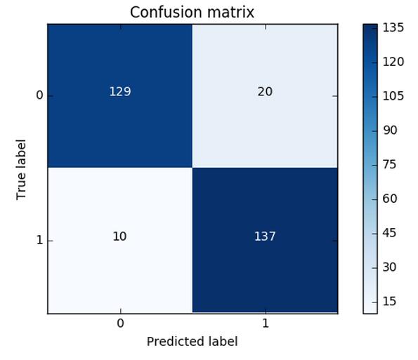

这个图就非常漂亮了！（并不是说画的好而是展示的很直接）从图中可以清晰的看到原始数据中样本的分布以及我们的模型的预测结果，那么recall是怎么算出来的呢？就是用我们的检测到的个数（137）去除以总共异常样本的个数（10+137），用这个数值来去评估我们的模型。利用混淆矩阵我们可以很直观的考察模型的精度以及recall，也是非常推荐大家在评估模型的时候不妨把这个图亮出来可以帮助咱们很直观的看清楚现在模型的效果以及存在的问题。

lr = LogisticRegression(C = best_c, penalty = 'l1')
lr.fit(X_train_undersample,y_train_undersample.values.ravel())
y_pred = lr.predict(X_test.values)

# Compute confusion matrix
cnf_matrix = confusion_matrix(y_test,y_pred)
np.set_printoptions(precision=2)

print("Recall metric in the testing dataset: ", cnf_matrix[1,1]/(cnf_matrix[1,0]+cnf_matrix[1,1]))

# Plot non-normalized confusion matrix
class_names = [0,1]
plt.figure()
plot_confusion_matrix(cnf_matrix
                      , classes=class_names
                      , title='Confusion matrix')
plt.show()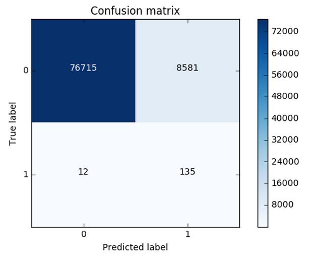

这可还木有完事，我们刚才只是在下采样的数据集中去进行测试的，那么这份测试还不能完全可信，因为它并不是原始的测试集，我们需要在原始的，大量的测试集中再次去衡量当前模型的效果。可以看到效果其实还不错，但是哪块有些问题呢，是不是我们误杀了很多呀，有些样本并不是异常的，但是并我们错误的当成了异常的，这个现象其实就是下采样策略本身的一个缺陷。

对于逻辑回归算法来说，我们还可以指定这样一个阈值，也就是说最终结果的概率是大于多少我们把它当成是正或者负样本。不用的阈值会对结果产生很大的影响。

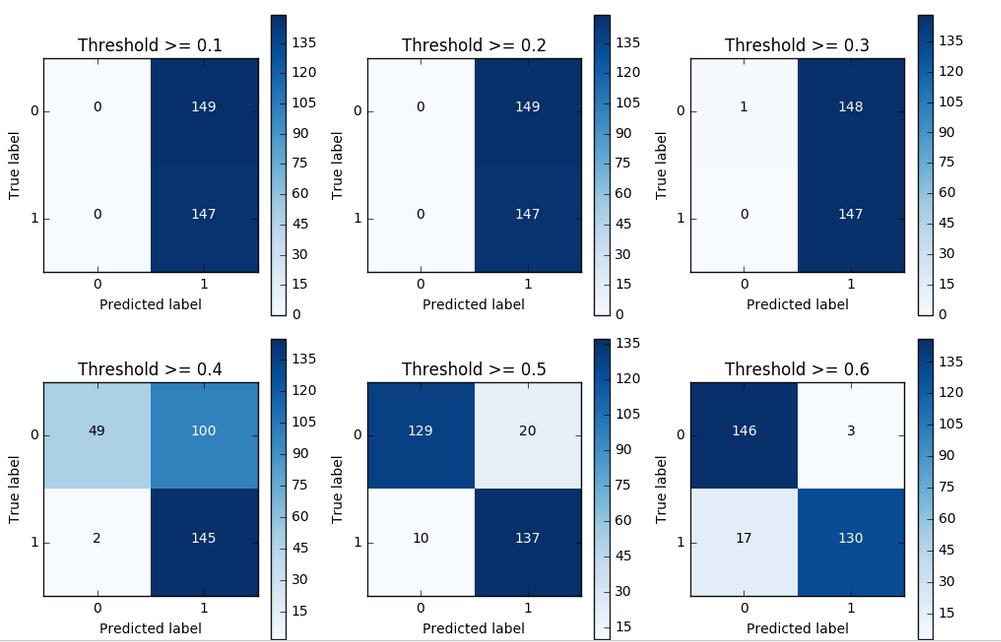
上图中我们可以看到不用的阈值产生的影响还是蛮大的，阈值较小，意味着我们的模型非常严格宁肯错杀也不肯放过，这样会使得绝大多数样本都被当成了异常的样本，recall很高，精度稍低 当阈值较大的时候我们的模型就稍微宽松些啦，这个时候会导致recall很低，精度稍高，综上当我们使用逻辑回归算法的时候，还需要根据实际的应用场景来选择一个最恰当的阈值！

说完了下采样策略，我们继续唠一下过采样策略，跟下采样相反，现在咱们的策略是要让class为0和1的样本一样多，也就是我们需要去进行数据的生成啦!

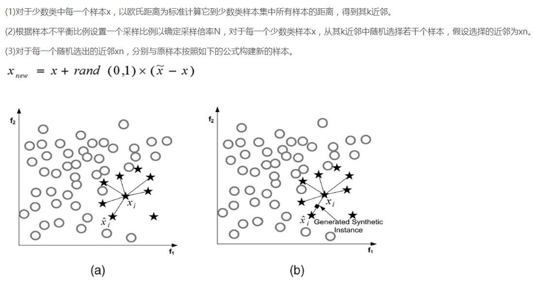
SMOTE算法是用的非常广泛的数据生成策略，流程可以参考上图，还是非常简单的，下面我们使用现成的库来帮助我们完成过采样数据生成策略。

import pandas as pd
from imblearn.over_sampling import SMOTE
from sklearn.ensemble import RandomForestClassifier
from sklearn.metrics import confusion_matrix
from sklearn.model_selection import train_test_split

credit_cards=pd.read_csv('creditcard.csv')

columns=credit_cards.columns
# The labels are in the last column ('Class'). Simply remove it to obtain features columns
features_columns=columns.delete(len(columns)-1)

features=credit_cards[features_columns]
labels=credit_cards['Class']

features_train, features_test, labels_train, labels_test = train_test_split(features, 
                                                                            labels, 
                                                                            test_size=0.2, 
                                                                            random_state=0)

oversampler=SMOTE(random_state=0)
os_features,os_labels=oversampler.fit_sample(features_train,labels_train)

很简单的几步操作我们就完成过采样策略，那么现在正负样本就是一样多的啦，都有那么20多W个，现在我们再通过混淆矩阵来看一下，逻辑回归应用于过采样样本的效果。数据增强的应用面已经非常广了，对于很多机器学习或者深度学习问题，这已经成为了一个常规套路啦！

我们对比一下下采样和过采样的效果，可以说recall的效果都不错，都可以检测到异常样本，但是下采样是不是误杀的比较少呀，所以如果我们可以进行数据生成，那么在处理样本数据不均衡的情况下，过采样是一个可以尝试的方案！

总结：

对于一个机器学习案例来说，一份数据肯定伴随着很多的挑战和问题，那么最为重要的就是我们该怎么解决这一系列的问题，大牛们不见得代码写的比咱们强但是他们却很清楚如何去解决问题。今天我们讲述了一个以检测任务为背景的案例，其中涉及到如何处理样本不均衡问题，以及模型评估选择的方法，最后给出了逻辑回归在不用阈值下的结果。这里也是希望大家可以通过案例多多积攒经验，早日成为技术大牛。