机器学习 决策树算法 (Decision Tree)

____tz_zs学习笔记

 

决策树算法概念：

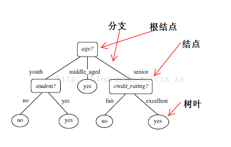
决策树（decision tree）是一个类似于流程图的树结构：其中，每个内部结点表示在一个属性上的测试，每个分支代表一个属性输出，而每个树叶结点代表类或类分布。树的最顶层是根结点。

 

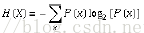
熵（entropy）概念：

决策树归纳算法（ID3）：

 

1970-1980，J.Ross.Quinlan，ID3算法

          选择属性判断结点

          信息获取量(Information Gain)：Gain(A) = Info(D) - Infor_A(D)

          通过一个来作为节点分类获取了多少信息

 

 

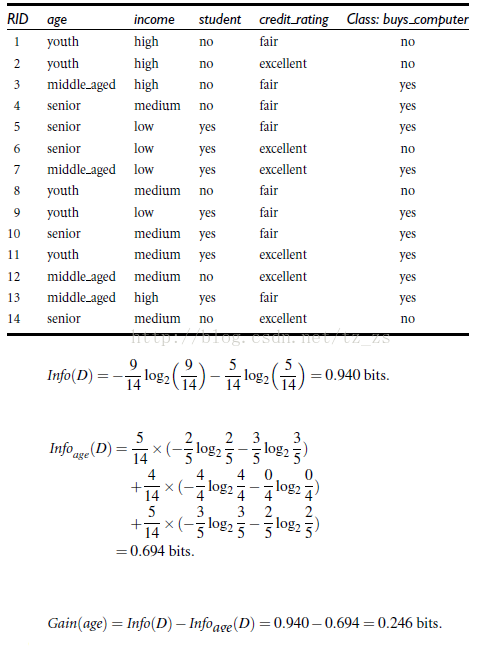
           类似，Gain(income) = 0.029, Gain(student) = 0.151, Gain(credit_rating)=0.048

          所以，选择age作为第一个根节点

.

 

sklearn.tree.DecisionTreeClassifier

基于 scikit-learn 的决策树分类模型 DecisionTreeClassifier 进行的分类运算

http://scikit-learn.org/stable/modules/generated/sklearn.tree.DecisionTreeClassifier.html#sklearn.tree.DecisionTreeClassifier

class sklearn.tree.DecisionTreeClassifier(criterion=’gini’, splitter=’best’, max_depth=None, min_samples_split=2, min_samples_leaf=1, min_weight_fraction_leaf=0.0, max_features=None, random_state=None, max_leaf_nodes=None, min_impurity_decrease=0.0, min_impurity_split=None, class_weight=None, presort=False)

参数：

criterion : 默认为 "gini"。是特征选择的标准，可选择基尼系数 "gini" 或者 信息熵 "entropy"。

splitter : 默认为 "best"。"best" 是在特征的所有划分点中找出最优的划分点。"random" 是随机的在部分划分点中找局部最优的划分点。"best" 适合样本量不大的时候，如果样本数据量非常大，推荐 "random"。

max_depth : 默认为 None。设置树的最大深度。如果是 None，则不限制子树的深度，直到所有叶子是纯的，或者所有叶子包含少于 min_samples_split 的样本。

min_samples_split : 默认为 2，可以是 int 或者 float 格式。限制子树继续划分的条件，如果节点的样本数小于这个值，则不会再划分。当为 float 值时，拆分的最小样本数为 ceil(min_samples_split * n_samples)。

min_samples_leaf : 默认为1，可以是 int 或者 float 格式。设置叶子节点的最小样本数，如果某叶子节点数目小于样本数，则会和兄弟节点一起被剪枝。当为 float 值时，此时叶子最小样本数为 ceil（min_samples_leaf * n_samples）。

min_weight_fraction_leaf : 叶子节点最小的样本权重和。这个值限制了叶子节点所有样本权重和的最小值，如果小于这个值，则会和兄弟节点一起被剪枝。 默认是0，就是不考虑权重问题。一般来说，如果我们有较多样本有缺失值，或者分类树样本的分布类别偏差很大，就会引入样本权重，这时我们就要注意这个值了。

max_features : 划分时考虑的最大特征数，默认为 None。是划分时考虑的最大特征数，

• 如果是 int, 最大特征数为此 max_features 值。
• 如果是 float,  值为 int(max_features * n_features)。
• 如果是 “auto”, 值为 max_features=sqrt(n_features)。
• 如果是 “sqrt”, 值为 max_features=sqrt(n_features)。
• 如果是 “log2”, 值为 max_features=log2(n_features)。
• 如果是 None, 值为 max_features=n_features 表示划分时考虑所有的特征数。

random_state : 默认为 None。随机种子。

max_leaf_nodes : 最大叶子节点数，默认为 None。限制最大叶子节点数，可以防止过拟合如果为 None，则不显示最大的叶子节点数。

class_weight : 指定样本各类别的的权重。默认为 None，表示没有权重偏倚。如果为 "balanced"，则算法会自己计算权重，样本少的权重高，公式：n_samples / (n_classes * np.bincount(y))。

min_impurity_decrease : 默认为0。参数的意义是，如果继续分裂能减少的杂质大于或等于该值，则分裂节点。

min_impurity_split : 如果节点的不纯度高于阈值，节点将分裂。（已被 min_impurity_decrease 代替）。

presort : 设置数据是否预排序，默认为 False。在大型数据集上，设置为 True 可能反而会降低训练速度，在较小数据集或者限制深度的树上使用 True 能加快训练速度。

属性：

max_features_ : 特征的数量

feature_importances_ : 特征的重要性。

 

参考：

https://www.cnblogs.com/pinard/p/6056319.html

https://www.jianshu.com/p/78594737b4b4

.

 

示例代码：

网络课程中python2中的代码

from sklearn.feature_extraction import DictVectorizer
import csv
from sklearn import tree
from sklearn import preprocessing
from sklearn.externals.six import StringIO


# Read in the csv file and put features into list of dict and list of class label


allElectronicsData = open(r'/home/zhoumiao/MachineLearning/01decisiontree/AllElectronics.csv', 'rb')
reader = csv.reader(allElectronicsData)
headers = reader.next()


print(headers)


featureList = []
labelList = []


for row in reader:
    labelList.append(row[len(row)-1])
    rowDict = {}
    for i in range(1, len(row)-1):
        rowDict[headers[i]] = row[i]
    featureList.append(rowDict)


print(featureList)


# Vetorize features
vec = DictVectorizer()
dummyX = vec.fit_transform(featureList) .toarray()


print("dummyX: " + str(dummyX))
print(vec.get_feature_names())


print("labelList: " + str(labelList))


# vectorize class labels
lb = preprocessing.LabelBinarizer()
dummyY = lb.fit_transform(labelList)
print("dummyY: " + str(dummyY))


# Using decision tree for classification
# clf = tree.DecisionTreeClassifier()
clf = tree.DecisionTreeClassifier(criterion='entropy')
clf = clf.fit(dummyX, dummyY)
print("clf: " + str(clf))




# Visualize model
with open("allElectronicInformationGainOri.dot", 'w') as f:
    f = tree.export_graphviz(clf, feature_names=vec.get_feature_names(), out_file=f)


oneRowX = dummyX[0, :]
print("oneRowX: " + str(oneRowX))


newRowX = oneRowX
newRowX[0] = 1
newRowX[2] = 0
print("newRowX: " + str(newRowX))


predictedY = clf.predict(newRowX)
print("predictedY: " + str(predictedY))

.

python3要修改一些方法的使用规则。

代码逻辑：

①前一部分为读取文件

②将数据矢量化（变为0,1）

③之后训练决策树

④将决策树可视化：先写如点格式文件，然后使用Graphviz的软件转化为PDF格式

⑤使用决策树预测标签

# -*- coding: utf-8 -*-
"""
@author: tz_zs
"""


from sklearn.feature_extraction import DictVectorizer
import csv
from sklearn import tree
from sklearn import preprocessing
from sklearn.externals.six import StringIO


import numpy as np
np.set_printoptions(threshold = 1e6)#设置打印数量的阈值 


# Read in the csv file and put features into list of dict and list of class label
allElectronicsData = open(r'AllElectronics.csv', 'r')
reader = csv.reader(allElectronicsData)
#headers = reader.next()
headers = next(reader)


print(headers)
print("~"*10+"headers end"+"~"*10)


featureList = []
labelList = []


for row in reader:  # 遍历每一列
    labelList.append(row[len(row)-1])   # 标签列表
    rowDict = {}                        # 每一行的所有特征放入一个字典
    for i in range(1, len(row)-1):      # 左闭右开 遍历从age到credit_rating
        rowDict[headers[i]] = row[i]    # 字典的赋值
    featureList.append(rowDict)         #将每一行的特征字典装入特征列表内


print(featureList)
print("~"*10+"featureList end"+"~"*10)


# Vetorize features
vec = DictVectorizer() # Vectorizer 矢量化
dummyX = vec.fit_transform(featureList).toarray()


print("dummyX: " + str(dummyX))
print(vec.get_feature_names())
print("~"*10+"dummyX end"+"~"*10)


print("labelList: " + str(labelList))
print("~"*10+"labelList end"+"~"*10)


# vectorize class labels
lb = preprocessing.LabelBinarizer()
dummyY = lb.fit_transform(labelList)
print("dummyY: " + str(dummyY))
print("~"*10+"dummyY end"+"~"*10)


# Using decision tree for classification
# clf = tree.DecisionTreeClassifier()
clf = tree.DecisionTreeClassifier(criterion='entropy')  # 标准 熵
clf = clf.fit(dummyX, dummyY)
print("clf: " + str(clf))




# Visualize model
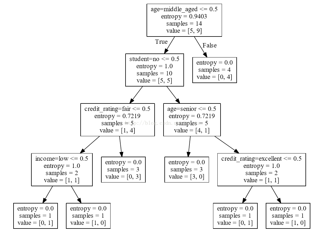
with open("allElectronicInformationGainOri.dot", 'w') as f:
    # 输出到dot文件里，安装 Graphviz软件后，
    # 可使用 dot -Tpdf allElectronicInformationGainOri.dot -o outpu.pdf 命令 
    # 转化dot文件至pdf可视化决策树
    f = tree.export_graphviz(clf, feature_names=vec.get_feature_names(), out_file=f)




oneRowX = dummyX[0, :]
print("oneRowX: " + str(oneRowX))


newRowX = oneRowX
newRowX[0] = 1
newRowX[2] = 0
print("newRowX: " + str(newRowX))


predictedY = clf.predict(newRowX)
print("predictedY: " + str(predictedY))

.

点文件内容：

有向图树{
node [shape = box];
0 [label =“age = middle_aged <= 0.5 \ nentropy = 0.9403 \ nsamples = 14 \ nvalue = [5，9]”];
1 [label =“student = yes <= 0.5 \ nentropy = 1.0 \ nsamples = 10 \ nvalue = [5，5]”];
0  - > 1 [labeldistance = 2.5，labelangle = 45，headlabel =“True”];
2 [label =“age = senior <= 0.5 \ nentropy = 0.7219 \ nsamples = 5 \ nvalue = [4，1]”];
1  - > 2;
3 [label =“entropy = 0.0 \ nsamples = 3 \ nvalue = [3，0]”];
2  - > 3;
4 [label =“credit_rating = excellent <= 0.5 \ nentropy = 1.0 \ nsamples = 2 \ nvalue = [1，1]”];
2  - > 4;
5 [label =“entropy = 0.0 \ nsamples = 1 \ nvalue = [0，1]”];
4  - > 5;
6 [label =“entropy = 0.0 \ nsamples = 1 \ nvalue = [1，0]”];
4  - > 6;
7 [label =“credit_rating = excellent <= 0.5 \ nentropy = 0.7219 \ nsamples = 5 \ nvalue = [1，4]”];
1  - > 7;
8 [label =“entropy = 0.0 \ nsamples = 3 \ nvalue = [0，3]”];
7  - > 8;
9 [label =“income = medium <= 0.5 \ nentropy = 1.0 \ nsamples = 2 \ nvalue = [1，1]”];
7  - > 9;
10 [label =“entropy = 0.0 \ nsamples = 1 \ nvalue = [1，0]”];
9  - > 10;
11 [label =“entropy = 0.0 \ nsamples = 1 \ nvalue = [0，1]”];
9  - > 11;
12 [label =“entropy = 0.0 \ nsamples = 4 \ nvalue = [0，4]”];
0  - > 12 [labeldistance = 2.5，labelangle = -45，headlabel =“False”];
}

.

PDF内容：

 

代码运行输出：

['RID', 'age', 'income', 'student', 'credit_rating', 'class_buys_computer']
~~~~~~~~~~headers end~~~~~~~~~~
[{'age': 'youth', 'income': 'high', 'student': 'no', 'credit_rating': 'fair'}, {'age': 'youth', 'income': 'high', 'student': 'no', 'credit_rating': 'excellent'}, {'age': 'middle_aged', 'income': 'high', 'student': 'no', 'credit_rating': 'fair'}, {'age': 'senior', 'income': 'medium', 'student': 'no', 'credit_rating': 'fair'}, {'age': 'senior', 'income': 'low', 'student': 'yes', 'credit_rating': 'fair'}, {'age': 'senior', 'income': 'low', 'student': 'yes', 'credit_rating': 'excellent'}, {'age': 'middle_aged', 'income': 'low', 'student': 'yes', 'credit_rating': 'excellent'}, {'age': 'youth', 'income': 'medium', 'student': 'no', 'credit_rating': 'fair'}, {'age': 'youth', 'income': 'low', 'student': 'yes', 'credit_rating': 'fair'}, {'age': 'senior', 'income': 'medium', 'student': 'yes', 'credit_rating': 'fair'}, {'age': 'youth', 'income': 'medium', 'student': 'yes', 'credit_rating': 'excellent'}, {'age': 'middle_aged', 'income': 'medium', 'student': 'no', 'credit_rating': 'excellent'}, {'age': 'middle_aged', 'income': 'high', 'student': 'yes', 'credit_rating': 'fair'}, {'age': 'senior', 'income': 'medium', 'student': 'no', 'credit_rating': 'excellent'}]
~~~~~~~~~~featureList end~~~~~~~~~~
dummyX: [[ 0.  0.  1.  0.  1.  1.  0.  0.  1.  0.]
 [ 0.  0.  1.  1.  0.  1.  0.  0.  1.  0.]
 [ 1.  0.  0.  0.  1.  1.  0.  0.  1.  0.]
 [ 0.  1.  0.  0.  1.  0.  0.  1.  1.  0.]
 [ 0.  1.  0.  0.  1.  0.  1.  0.  0.  1.]
 [ 0.  1.  0.  1.  0.  0.  1.  0.  0.  1.]
 [ 1.  0.  0.  1.  0.  0.  1.  0.  0.  1.]
 [ 0.  0.  1.  0.  1.  0.  0.  1.  1.  0.]
 [ 0.  0.  1.  0.  1.  0.  1.  0.  0.  1.]
 [ 0.  1.  0.  0.  1.  0.  0.  1.  0.  1.]
 [ 0.  0.  1.  1.  0.  0.  0.  1.  0.  1.]
 [ 1.  0.  0.  1.  0.  0.  0.  1.  1.  0.]
 [ 1.  0.  0.  0.  1.  1.  0.  0.  0.  1.]
 [ 0.  1.  0.  1.  0.  0.  0.  1.  1.  0.]]
['age=middle_aged', 'age=senior', 'age=youth', 'credit_rating=excellent', 'credit_rating=fair', 'income=high', 'income=low', 'income=medium', 'student=no', 'student=yes']
~~~~~~~~~~dummyX end~~~~~~~~~~
labelList: ['no', 'no', 'yes', 'yes', 'yes', 'no', 'yes', 'no', 'yes', 'yes', 'yes', 'yes', 'yes', 'no']
~~~~~~~~~~labelList end~~~~~~~~~~
dummyY: [[0]
 [0]
 [1]
 [1]
 [1]
 [0]
 [1]
 [0]
 [1]
 [1]
 [1]
 [1]
 [1]
 [0]]
~~~~~~~~~~dummyY end~~~~~~~~~~
clf: DecisionTreeClassifier(class_weight=None, criterion='entropy', max_depth=None,
            max_features=None, max_leaf_nodes=None,
            min_impurity_split=1e-07, min_samples_leaf=1,
            min_samples_split=2, min_weight_fraction_leaf=0.0,
            presort=False, random_state=None, splitter='best')
oneRowX: [ 0.  0.  1.  0.  1.  1.  0.  0.  1.  0.]
newRowX: [ 1.  0.  0.  0.  1.  1.  0.  0.  1.  0.]
predictedY: [1]

.

补充：

发现有不少小伙伴在 dot 转 PDF 时遇到了 dot 或 GraphViz 找不到等等问题。这里有几点提醒：

一、注意在Python中安装好 GraphViz （pip install graphviz）和 pydot （pip install pydot）三方库后，你还需要下载 GraphViz（https://www.graphviz.org/）软件安装。（Linux 可以在终端使用命令 sudo apt-get install graphviz 安装）

二、很可能是因为没把graphviz的bin目录加入path路径。

三、注意先安装 GraphViz，再安装 pydot。

参考：

• https://www.bbsmax.com/A/B0zqBekNJv/
• https://stackoverflow.com/questions/27666846/pydot-invocationexception-graphvizs-executables-not-found
• https://stackoverflow.com/questions/18438997/why-is-pydot-unable-to-find-graphvizs-executables-in-windows-8

.

end