Xgboost参数调优的完整指南及实战

小虎AI实验室

已于 2022-05-10 16:32:00 修改

阅读量6.1w

点赞数 84

分类专栏： Machine_learning 机器学习文章标签： Xgboost Tuning parameter CV

于 2017-11-14 17:09:34 首次发布

本文链接：https://blog.csdn.net/u010665216/article/details/78532619

版权

Machine_learning 同时被 2 个专栏收录

58 篇文章 41 订阅

订阅专栏

机器学习

51 篇文章 28 订阅

订阅专栏

引言

Xgboost是一种高度复杂的算法可以处理各种各样的数据。相信每个用过Xgboost的人都有过这样的感受：利用Xgboost构建模型十分简单，但是用Xgboost来调参提升模型就很难了。该算法使用多个参数。为了改进模型，必须对参数进行优化。但是我们很难找到实际问题的答案——你应该调整哪些参数?这些参数的理想值是什么?以前我写过一篇Xgboost与lightgbm参数对比的文章，但是感觉应该把Xgboost、lightgbm参数调优独立成两篇文章详细说明下，这样既能自己作为日后查看的笔记，又能与大家一起分享自己的理解。
在本文中，我们将学习关于XGBoost的一些有用信息的参数调优技术。此外，我们还将使用Python中的数据集实践该算法。

Xgboost的优势

有关Xgboost的前世今生，请戳：传送门。Xgboost在预测任务中有着极其强大的能力，深究其性能与背后的机理，我们总结出以下几个优势：
1.Regularization（正则化）:

Xgboost就是一个以”正则化提升“技术闻名的工具，很明显，这可以减少过拟合。

2.Parallel Processing（并行处理）:

如果大家看过我前面分享的一篇集成学习的文章：集成学习之bagging、boosting及AdaBoost的实现不免心生疑问，那篇文章中明确指出，boosting算法是串行算法，每个学习器的生成都是依赖于前面一个学习器的生成的，那么Xgboost又是如何实现并行的呢，详情请戳：Parallel Gradient Boosting Decision Trees。

3.High Flexibility（高度灵活）：

Xgboost可以让使用者自定义优化目标与评估标准。

4.Handling Missing Values（处理缺失值）：

Xgboost通过一个内置的程序来处理缺失值，但是需要用户提供一个与其他观察值不同的缺失值，并作为参数传递。

5.Tree Pruning（树剪枝）:

Xgboost中有个参数max_depth，因此Xgboost会持续分裂直到达到max_depth，然后回溯剪枝

6.Built-in Cross-Validation（内置的交叉验证）：

Xgboost允许用户在每次boosting迭代的过程中应用交叉验证

8.Continue on Existing Model（继续现有模型）：

用户可以从上一次运行的最后一次迭代中开始训练XGBoost模型。这在某些特定的应用程序中具有很大的优势。

Xgboost的参数

Xgboost的作者将工具分成了三大类：

General Parameters（通用参数）：设置整体功能
Booster Parameters（提升参数）：选择你每一步的booster(树or回归）
Learning Task Parameters（学习任务参数）：指导优化任务的执行

通用参数

下面这些参数定义了Xgboost的总体功能：
1.booster [default=gbtree]

选择每次迭代过程中需要运行的模型，一共有两种选择：
gbtree: tree-based models

2.silent [default=0]

设置模型是否有logo打印：
0：有打印
1：无打印

3.nthread [default to maximum number of threads available if not set]

这个主要用于并行处理的，如果不指定值，工具会自动检测

剩余两个参数是Xgboost自动指定的，无需设置

提升参数

虽然有两种类型的booster，但是我们这里只介绍tree。因为tree的性能比线性回归好得多，因此我们很少用线性回归。
1.eta [default=0.3, alias: learning_rate]

学习率，可以缩减每一步的权重值，使得模型更加健壮：
典型值一般设置为：0.01-0.2

2.min_child_weight [default=1]

定义了一个子集的所有观察值的最小权重和。
这个可以用来减少过拟合，但是过高的值也会导致欠拟合，因此可以通过CV来调整min_child_weight。

3.max_depth [default=6]

树的最大深度，值越大，树越复杂。
这个可以用来控制过拟合，典型值是3-10。

4.gamma [default=0, alias: min_split_loss]

这个指定了一个结点被分割时，所需要的最小损失函数减小的大小。
这个值一般来说需要根据损失函数来调整。

5.max_delta_step(默认= 0)

这个参数通常并不需要。

6.subsample [default=1]

样本的采样率，如果设置成0.5，那么Xgboost会随机选择一般的样本作为训练集。

7.colsample_bytree [default=1]

构造每棵树时，列采样率（一般是特征采样率）。

8.colsample_bylevel [default=1]

每执行一次分裂，列采样率。这个一般很少用，6和7参数调节就足够了。

9.lambda [default=1, alias: reg_lambda]

L2正则化（与岭回归中的正则化类似：传送门）这个其实用的很少。

10.alpha [default=0, alias: reg_alpha]

L1正则化（与lasso回归中的正则化类似：传送门）这个主要是用在数据维度很高的情况下，可以提高运行速度。

11.scale_pos_weight, [default=1]

在类别高度不平衡的情况下，将参数设置大于0，可以加快收敛。

学习任务参数

这类参数主要用来明确学习任务和相应的学习目标的
1.objective [default=reg:linear]

这个主要是指定学习目标的：而分类，还是多分类or回归
“reg:linear” –linear regression：回归
“binary:logistic”：二分类
“multi:softmax” ：多分类，这个需要指定类别个数

2.eval_metric [default according to objective]

*评估方法，主要用来验证数据，根据一个学习目标会默认分配一个评估指标
“rmse”:均方根误差（回归任务）
“error”:分类任务
“map”:Mean average precision（平均准确率，排名任务）
等等

3.seed [default=0]

随机数种子，可以用来生成可复制性的结果，也可用来调参

Xgboost参数调优实例

这里我们从一个网上找到一份数据集，数据集预先被我处理过，data与code均可在gitee上下载。

调参的通用方法

选择一个相对较高的学习率。通常来说学习率设置为0.1。但是对于不同的问题可以讲学习率设置在0.05-0.3。通过交叉验证来寻找符合学习率的最佳树的个数。
当确定好学习率与最佳树的个数时，调整树的某些特定参数。比如：max_depth, min_child_weight, gamma, subsample, colsample_bytree
调整正则化参数，比如： lambda, alpha。这个主要是为了减少模型复杂度和提高运行速度的。适当地减少过拟合。
降低学习速率，选择最优参数

接下来，我们通过实际例子来一步一步地调参并分析

step1.修正学习速率及调参估计量

首先我们设置一些参数的初始值(你可以设置不同的值）：

max_depth = 5
min_child_weight = 1
gamma = 0
subsample, colsample_bytree = 0.8
scale_pos_weight = 1

具体参数如下：

#Choose all predictors except target & IDcols
predictors = [x for x in train.columns if x not in [target, IDcol]]
xgb1 = XGBClassifier(
 learning_rate =0.1,
 n_estimators=20,
 max_depth=5,
 min_child_weight=1,
 gamma=0,
 subsample=0.8,
 colsample_bytree=0.8,
 objective= 'binary:logistic',
 nthread=4,
 scale_pos_weight=1,
 seed=27)
modelfit(xgb1, train, predictors)

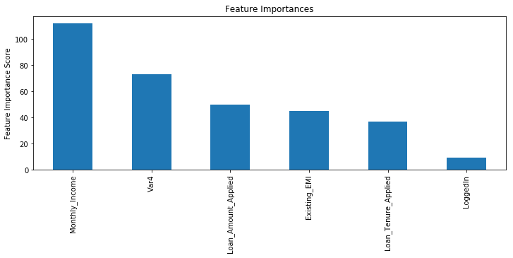
我们来看下输出的结果：

[out] :
Model Report
Accuracy : 0.6084
AUC Score (Train): 0.652469

step1

step2.调整max_depth 和min_child_weight

我们调整这两个参数是因为这两个参数对输出结果的影响很大。我们首先将这两个参数设置为较大的数，然后通过迭代的方式不断修正，缩小范围。（接下来的网格搜索，会消耗很多时间）

param_test1 = {
 'max_depth':list(range(3,10,2)),
 'min_child_weight':list(range(1,6,2))
}
gsearch1 = GridSearchCV(estimator = XGBClassifier( learning_rate =0.1, n_estimators=20, max_depth=5,
 min_child_weight=1, gamma=0, subsample=0.8, colsample_bytree=0.8,
 objective= 'binary:logistic', nthread=4, scale_pos_weight=1, seed=27), 
 param_grid = param_test1, scoring='roc_auc',n_jobs=4,iid=False, cv=5)
gsearch1.fit(train[predictors],train[target])
gsearch1.grid_scores_, gsearch1.best_params_, gsearch1.best_score_

这里我们选择两个序列‘max_depth’范围3-10步长2；’min_child_weight’范围1-6，步长2。
这样两两组合就有12种组合方式。输出结果如下：

[out]:
([mean: 0.59883, std: 0.00449, params: {'max_depth': 3, 'min_child_weight': 1},
  mean: 0.59888, std: 0.00450, params: {'max_depth': 3, 'min_child_weight': 3},
  mean: 0.59889, std: 0.00450, params: {'max_depth': 3, 'min_child_weight': 5},
  mean: 0.64832, std: 0.00346, params: {'max_depth': 5, 'min_child_weight': 1},
  mean: 0.64876, std: 0.00320, params: {'max_depth': 5, 'min_child_weight': 3},
  mean: 0.64830, std: 0.00317, params: {'max_depth': 5, 'min_child_weight': 5},
  mean: 0.66681, std: 0.00345, params: {'max_depth': 7, 'min_child_weight': 1},
  mean: 0.66649, std: 0.00330, params: {'max_depth': 7, 'min_child_weight': 3},
  mean: 0.66635, std: 0.00350, params: {'max_depth': 7, 'min_child_weight': 5},
  mean: 0.67342, std: 0.00310, params: {'max_depth': 9, 'min_child_weight': 1},
  mean: 0.67320, std: 0.00325, params: {'max_depth': 9, 'min_child_weight': 3},
  mean: 0.67303, std: 0.00284, params: {'max_depth': 9, 'min_child_weight': 5}],
 {'max_depth': 9, 'min_child_weight': 1},
 0.6734158281875513)

其中最佳组合方式是:{‘max_depth’: 9, ‘min_child_weight’: 1}
接下来缩小范围，将两个序列范围约束在[8,10,1];[1,2,1]

param_test2 = {
 'max_depth':[8,9,10],
 'min_child_weight':[1,2,3]
}
gsearch2 = GridSearchCV(estimator = XGBClassifier( learning_rate=0.1, n_estimators=20, max_depth=5,
 min_child_weight=2, gamma=0, subsample=0.8, colsample_bytree=0.8,
 objective= 'binary:logistic', nthread=4, scale_pos_weight=1,seed=27), 
 param_grid = param_test2, scoring='roc_auc',n_jobs=4,iid=False, cv=5)
gsearch2.fit(train[predictors],train[target])
gsearch2.grid_scores_, gsearch2.best_params_, gsearch2.best_score_

我们再来看输出结果：

[out]:
([mean: 0.67118, std: 0.00354, params: {'max_depth': 8, 'min_child_weight': 1},
  mean: 0.67088, std: 0.00327, params: {'max_depth': 8, 'min_child_weight': 2},
  mean: 0.67070, std: 0.00332, params: {'max_depth': 8, 'min_child_weight': 3},
  mean: 0.67342, std: 0.00310, params: {'max_depth': 9, 'min_child_weight': 1},
  mean: 0.67299, std: 0.00308, params: {'max_depth': 9, 'min_child_weight': 2},
  mean: 0.67320, std: 0.00325, params: {'max_depth': 9, 'min_child_weight': 3},
  mean: 0.67469, std: 0.00303, params: {'max_depth': 10, 'min_child_weight': 1},
  mean: 0.67421, std: 0.00307, params: {'max_depth': 10, 'min_child_weight': 2},
  mean: 0.67411, std: 0.00282, params: {'max_depth': 10, 'min_child_weight': 3}],
 {'max_depth': 10, 'min_child_weight': 1},
 0.6746894769116867)

这里我们发现max_depth发生了变化，而且CV scores相较于前一个提高了。

step3.调整gamma

现在我们可以基于上面确定好的最优值来调整gamma值。

param_test3 = {
 'gamma':[i/10.0 for i in range(0,5)]
}
gsearch3 = GridSearchCV(estimator = XGBClassifier( learning_rate =0.1, n_estimators=20, max_depth=10,
 min_child_weight=1, gamma=0, subsample=0.8, colsample_bytree=0.8,
 objective= 'binary:logistic', nthread=4, scale_pos_weight=1,seed=27), 
 param_grid = param_test3, scoring='roc_auc',n_jobs=4,iid=False, cv=5)
gsearch3.fit(train[predictors],train[target])
gsearch3.grid_scores_, gsearch3.best_params_, gsearch3.best_score_

我们来看下输出：

[out]:
([mean: 0.67469, std: 0.00303, params: {'gamma': 0.0},
  mean: 0.67470, std: 0.00288, params: {'gamma': 0.1},
  mean: 0.67471, std: 0.00283, params: {'gamma': 0.2},
  mean: 0.67458, std: 0.00295, params: {'gamma': 0.3},
  mean: 0.67445, std: 0.00314, params: {'gamma': 0.4}],
 {'gamma': 0.2},
 0.6747090662657905)

这里gamma已经从我们前面默认的0，变成了0.2了

最后我们用最优参数再次运行一下程序：

xgb1 = XGBClassifier(
 learning_rate =0.1,
 n_estimators=20,
 max_depth=10,
 min_child_weight=1,
 gamma=0.2,
 subsample=0.8,
 colsample_bytree=0.8,
 objective= 'binary:logistic',
 nthread=4,
 scale_pos_weight=1,
 seed=27)
modelfit(xgb1, train, predictors)

[out]:
Model Report
Accuracy : 0.6403
AUC Score (Train): 0.703964

step3
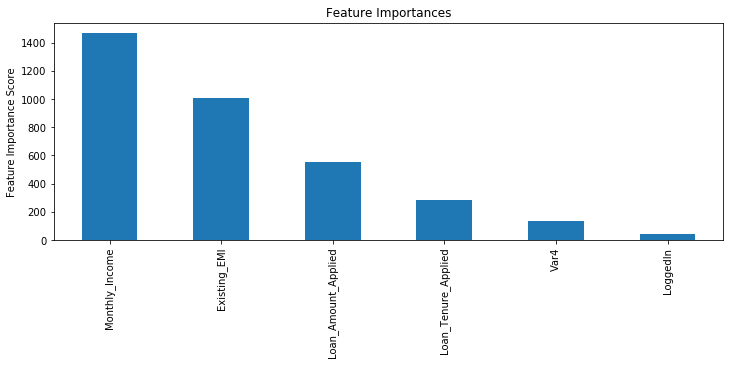
我们可以明显看到效果的提升。因此最终的参数是：

max_depth: 4
min_child_weight: 6
gamma: 0

step4.调整subsample 和colsample_bytree

这里我们方法如上

param_test5 = {
 'subsample':[i/100.0 for i in range(75,90,5)],
 'colsample_bytree':[i/100.0 for i in range(75,90,5)]
}
gsearch5 = GridSearchCV(estimator = XGBClassifier( learning_rate =0.1, n_estimators=20, max_depth=10,
 min_child_weight=1, gamma=0.2, subsample=0.8, colsample_bytree=0.8,
 objective= 'binary:logistic', nthread=4, scale_pos_weight=1,seed=27), 
 param_grid = param_test5, scoring='roc_auc',n_jobs=4,iid=False, cv=5)
gsearch5.fit(train[predictors],train[target])
gsearch5.grid_scores_, gsearch5.best_params_, gsearch5.best_score_

输出结果

[out]:
([mean: 0.67484, std: 0.00337, params: {'colsample_bytree': 0.75, 'subsample': 0.75},
  mean: 0.67471, std: 0.00283, params: {'colsample_bytree': 0.75, 'subsample': 0.8},
  mean: 0.67496, std: 0.00296, params: {'colsample_bytree': 0.75, 'subsample': 0.85},
  mean: 0.67484, std: 0.00337, params: {'colsample_bytree': 0.8, 'subsample': 0.75},
  mean: 0.67471, std: 0.00283, params: {'colsample_bytree': 0.8, 'subsample': 0.8},
  mean: 0.67496, std: 0.00296, params: {'colsample_bytree': 0.8, 'subsample': 0.85},
  mean: 0.67583, std: 0.00244, params: {'colsample_bytree': 0.85, 'subsample': 0.75},
  mean: 0.67543, std: 0.00281, params: {'colsample_bytree': 0.85, 'subsample': 0.8},
  mean: 0.67610, std: 0.00248, params: {'colsample_bytree': 0.85, 'subsample': 0.85}],
 {'colsample_bytree': 0.85, 'subsample': 0.85},
 0.6761040596420693)

step5.调整正则化参数

这个主要来调整过拟合，其实这个参数用的比较少，但是这里还是提供了一个样例：

param_test6 = {
 'reg_alpha':[1e-5, 1e-2, 0.1, 1, 100]
}
gsearch6 = GridSearchCV(estimator = XGBClassifier( learning_rate =0.1, n_estimators=20, max_depth=10,
 min_child_weight=1, gamma=0.2, subsample=0.8, colsample_bytree=0.8,
 objective= 'binary:logistic', nthread=4, scale_pos_weight=1,seed=27), 
 param_grid = param_test6, scoring='roc_auc',n_jobs=4,iid=False, cv=5)
gsearch6.fit(train[predictors],train[target])
gsearch6.grid_scores_, gsearch6.best_params_, gsearch6.best_score_

输出结果：

[out]:
([mean: 0.67471, std: 0.00283, params: {'reg_alpha': 1e-05},
  mean: 0.67487, std: 0.00298, params: {'reg_alpha': 0.01},
  mean: 0.67455, std: 0.00293, params: {'reg_alpha': 0.1},
  mean: 0.67468, std: 0.00308, params: {'reg_alpha': 1},
  mean: 0.66111, std: 0.00301, params: {'reg_alpha': 100}],
 {'reg_alpha': 0.01},
 0.6748686269296913)

接下来可以给reg_alpha选择精度更高的值，方法一样。
最终我实验的结果：

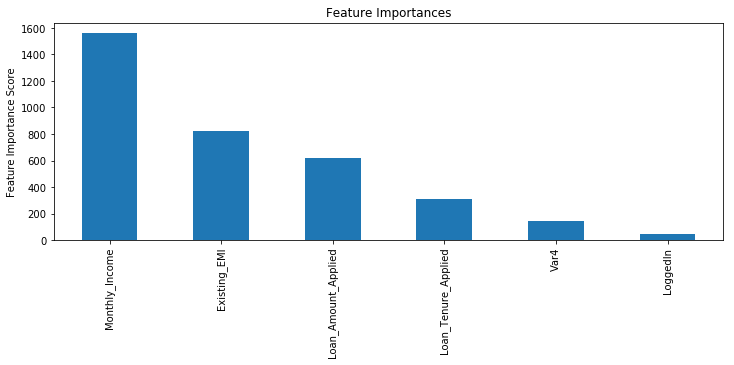
[out]:

Model Report
Accuracy : 0.6421
AUC Score (Train): 0.704268

res

step6.减小学习率

现在我们进一步降低学习率并增加树的数量

xgb4 = XGBClassifier(
 learning_rate =0.01,
 n_estimators=100,
 max_depth=10,
 min_child_weight=1,
 gamma=0.2,
 subsample=0.85,
 colsample_bytree=0.85,
 objective= 'binary:logistic',
 reg_alpha=0.01,
 nthread=4,
 scale_pos_weight=1,
 seed=27)
modelfit(xgb4, train, predictors)

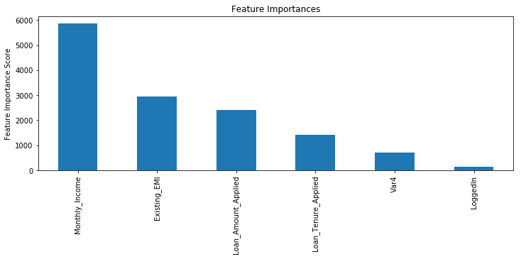
输出结果：

[out]:
Model Report
Accuracy : 0.6506
AUC Score (Train): 0.717132

last

总结

到这里我们参数调优就分享结束了。在结束这次分享之前，我想要给大家说明的是：**不要幻想仅仅通过参数调优或者换一个稍微更好的模型使得最终结果有巨大的飞跃。**要想最后的结果有巨大的提升，可以通过特征工程、模型集成来实现。

小虎AI实验室

关注

84
点赞
踩
633

收藏

觉得还不错? 一键收藏
打赏
12
评论
Xgboost参数调优的完整指南及实战

引言Xgboost是一种高度复杂的算法可以处理各种各样的数据。相信每个用过Xgboost的人都有过这样的感受：利用Xgboost构建模型十分简单，但是用Xgboost来调参提升模型就很难了。该算法使用多个参数。为了改进模型，必须对参数进行优化。但是我们很难找到实际问题的答案——你应该调整哪些参数?这些参数的理想值是什么?以前我写过一篇Xgboost与lightgbm参数对比的文章，但是感觉应该把Xg
复制链接

扫一扫