Deep learning-------------Neural networks

最新推荐文章于 2023-07-31 17:28:51 发布

jingruixiaozhuang

最新推荐文章于 2023-07-31 17:28:51 发布

阅读量794

点赞数

分类专栏： Deep Learning

本文链接：https://blog.csdn.net/u012796064/article/details/17069839

版权

Deep Learning 专栏收录该内容

26 篇文章 2 订阅

订阅专栏

I explain it in English.

Neural Networks

Consider a supervised learning problem where we have access to labeled training examples $(x (i), y (i))$ . Neural networks give a way of defining a complex, non-linear form of hypotheses $h W, b (x)$ , with parameters $W, b$ that we can fit to our data.

To describe neural networks, we will begin by describing the simplest possible neural network, one which comprises a single "neuron." We will use the following diagram to denote a single neuron:

This "neuron" is a computational unit that takes as input $x 1, x 2, x 3$ (and a +1 intercept term), and outputs $\textstyle h_{W,b}(x) = f(W^Tx) = f(\sum_{i=1}^3 W_{i}x_i +b)$ , where $f : \Re \mapsto \Re$ is called the activation function. In these notes, we will choose $f(\cdot)$ to be the sigmoid function:

$f(z) = \frac{1}{1+\exp(-z)}.$

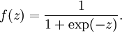
Thus, our single neuron corresponds exactly to the input-output mapping defined by logistic regression.

Although these notes will use the sigmoid function, it is worth noting that another common choice for $f$ is the hyperbolic tangent, or tanh, function:

$f(z) = \tanh(z) = \frac{e^z - e^{-z}}{e^z + e^{-z}},$

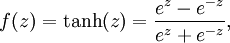
Here are plots of the sigmoid and $tanh$ functions:

The $tanh(z)$ function is a rescaled version of the sigmoid, and its output range is $[ - 1,1]$ instead of $[0,1]$ .

Note that unlike some other venues (including the OpenClassroom videos, and parts of CS229), we are not using the convention here of $x 0 = 1$ . Instead, the intercept term is handled separately by the parameter $b$ .

Finally, one identity that'll be useful later: If $f (z) = 1 / (1 + exp( - z))$ is the sigmoid function, then its derivative is given by $f'(z) = f (z)(1 - f (z))$ . (If $f$ is the tanh function, then its derivative is given by $f'(z) = 1 - (f (z)) 2$ .) You can derive this yourself using the definition of the sigmoid (or tanh) function.

Neural Network model

A neural network is put together by hooking together many of our simple "neurons," so that the output of a neuron can be the input of another. For example, here is a small neural network:

In this figure, we have used circles to also denote the inputs to the network. The circles labeled "+1" are called bias units, and correspond to the intercept term. The leftmost layer of the network is called the input layer, and the rightmost layer the output layer (which, in this example, has only one node). The middle layer of nodes is called thehidden layer, because its values are not observed in the training set. We also say that our example neural network has 3input units (not counting the bias unit), 3 hidden units, and 1 output unit.

We will let $n l$ denote the number of layers in our network; thus $n l = 3$ in our example. We label layer $l$ as $L l$ , so layer $L 1$ is the input layer, and layer $L_{n_l}$ the output layer. Our neural network has parameters $(W, b) = (W (1), b (1), W (2), b (2))$ , where we write $W^{(l)}_{ij}$ to denote the parameter (or weight) associated with the connection between unit $j$ in layer $l$ , and unit $i$ in layer $l + 1$ . (Note the order of the indices.) Also, $b^{(l)}_i$ is the bias associated with unit $i$ in layer $l + 1$ . Thus, in our example, we have $W^{(1)} \in \Re^{3\times 3}$ , and $W^{(2)} \in \Re^{1\times 3}$ . Note that bias units don't have inputs or connections going into them, since they always output the value +1. We also let $s l$ denote the number of nodes in layer $l$ (not counting the bias unit).

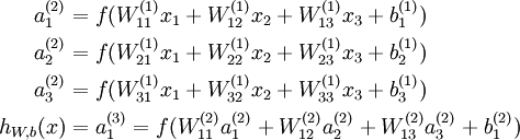
We will write $a^{(l)}_i$ to denote the activation (meaning output value) of unit $i$ in layer $l$ . For $l = 1$ , we also use $a^{(1)}_i = x_i$ to denote the $i$ -th input. Given a fixed setting of the parameters $W, b$ , our neural network defines a hypothesis $h W, b (x)$ that outputs a real number. Specifically, the computation that this neural network represents is given by:

$\begin{align}a_1^{(2)} &= f(W_{11}^{(1)}x_1 + W_{12}^{(1)} x_2 + W_{13}^{(1)} x_3 + b_1^{(1)}) \\a_2^{(2)} &= f(W_{21}^{(1)}x_1 + W_{22}^{(1)} x_2 + W_{23}^{(1)} x_3 + b_2^{(1)}) \\a_3^{(2)} &= f(W_{31}^{(1)}x_1 + W_{32}^{(1)} x_2 + W_{33}^{(1)} x_3 + b_3^{(1)}) \\h_{W,b}(x) &= a_1^{(3)} = f(W_{11}^{(2)}a_1^{(2)} + W_{12}^{(2)} a_2^{(2)} + W_{13}^{(2)} a_3^{(2)} + b_1^{(2)}) \end{align}$

In the sequel, we also let $z^{(l)}_i$ denote the total weighted sum of inputs to unit $i$ in layer $l$ , including the bias term (e.g., 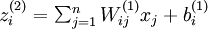$\textstyle z_i^{(2)} = \sum_{j=1}^n W^{(1)}_{ij} x_j + b^{(1)}_i$ ), so that $a^{(l)}_i = f(z^{(l)}_i)$ .

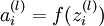Note that this easily lends itself to a more compact notation. Specifically, if we extend the activation function $f(\cdot)$ to apply to vectors in an element-wise fashion (i.e., $f ([z 1, z 2, z 3]) = [f (z 1), f (z 2), f (z 3)]$ ), then we can write the equations above more compactly as:

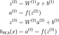
$\begin{align}z^{(2)} &= W^{(1)} x + b^{(1)} \\a^{(2)} &= f(z^{(2)}) \\z^{(3)} &= W^{(2)} a^{(2)} + b^{(2)} \\h_{W,b}(x) &= a^{(3)} = f(z^{(3)})\end{align}$

We call this step forward propagation. More generally, recalling that we also use $a (1) = x$ to also denote the values from the input layer, then given layer $l$ 's activations $a (l)$ , we can compute layer $l + 1$ 's activations $a (l + 1)$ as:

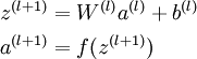
$\begin{align}z^{(l+1)} &= W^{(l)} a^{(l)} + b^{(l)} \\a^{(l+1)} &= f(z^{(l+1)})\end{align}$

By organizing our parameters in matrices and using matrix-vector operations, we can take advantage of fast linear algebra routines to quickly perform calculations in our network.

We have so far focused on one example neural network, but one can also build neural networks with other architectures(meaning patterns of connectivity between neurons), including ones with multiple hidden layers. The most common choice is a $\textstyle n_l$ -layered network where layer $\textstyle 1$ is the input layer, layer $\textstyle n_l$ is the output layer, and each layer $\textstyle l$ is densely connected to layer $\textstyle l+1$ . In this setting, to compute the output of the network, we can successively compute all the activations in layer $\textstyle L_2$ , then layer $\textstyle L_3$ , and so on, up to layer $\textstyle L_{n_l}$ , using the equations above that describe the forward propagation step. This is one example of a feedforward neural network, since the connectivity graph does not have any directed loops or cycles.

Neural networks can also have multiple output units. For example, here is a network with two hidden layers layers $L 2$ and $L 3$ and two output units in layer $L 4$ :

To train this network, we would need training examples $(x (i), y (i))$ where $y^{(i)} \in \Re^2$ . This sort of network is useful if there're multiple outputs that you're interested in predicting. (For example, in a medical diagnosis application, the vector $x$ might give the input features of a patient, and the different outputs $y i$ 's might indicate presence or absence of different diseases.)

本节内容: The representation and learning of neural networks

-----------------------The representation of neural networks-------------------------

（一）、为什么引入神经网络？——Nonlinear hypothesis

之前我们讨论的ML问题中，主要针对Regression做了分析，其中采用梯度下降法进行参数更新。然而其可行性基于假设参数不多，如果参数多起来了怎么办呢？比如下图中这个例子：从100*100个pixels中选出所有XiXj作为logistic regression的一个参数，那么总共就有5*10^7个feature，即x有这么多维。

所以引入了Nonlinear hypothesis，应对高维数据和非线性的hypothesis（如下图所示）：

===============================

（二）、神经元与大脑（neurons and brain）

神经元工作模式：

神经网络的逻辑单元：输入向量x（input layer），中间层a(2,i)（hidden layer）, 输出层h(x)（output layer）。

其中，中间层的a(2,i)中的2表示第二个级别（第一个级别是输入层），i表示中间层的第几个元素。或者可以说，a(j,i) is the activation of unit i in layer j.

===============================

（三）、神经网络的表示形式

从图中可知，中间层a(2，j)是输入层线性组合的sigmod值，输出又是中间层线性组合的sigmod值。

下面我们进行神经网络参数计算的向量化：

令z⁽²⁾表示中间层，x表示输入层，则有

，

z⁽²⁾=Θ⁽¹⁾x

a⁽²⁾=g(z⁽²⁾)

或者可以将x表示成a⁽¹⁾，那么对于输入层a⁽¹⁾有[x_0~x_3]4个元素，中间层a⁽²⁾有[a⁽²⁾₀~a⁽²⁾₃]4个元素（其中令a⁽²⁾₀=1），则有

h(x)= a⁽³⁾=g(z⁽³⁾)

z⁽³⁾=Θ⁽²⁾a⁽²⁾

通过以上这种神经元的传递方式（input->activation->output）来计算h(x), 叫做Forward propagation, 向前传递。

这里我们可以发现，其实神经网络就像是logistic regression，只不过我们把logistic regression中的输入向量[x₁~x₃]变成了中间层的[a⁽²⁾₁~a⁽²⁾₃], 即

h(x)=g(Θ⁽²⁾₀ a⁽²⁾₀+Θ⁽²⁾₁ a⁽²⁾₁+Θ⁽²⁾₂ a⁽²⁾₂+Θ⁽²⁾₃ a⁽²⁾₃)

而中间层又由真正的输入向量通过Θ⁽¹⁾学习而来，这里呢，就解放了输入层，换言之输入层可以是original input data的任何线性组合甚至是多项式组合如set x1*x2 as original x1...另外呢，具体怎样利用中间层进行更新下面会更详细地讲；此外，还有一些其他模型，比如：

===============================

（四）、怎样用神经网络实现逻辑表达式？

神经网路中，单层神经元（无中间层）的计算可用来表示逻辑运算，比如逻辑AND、逻辑或OR

举例说明：逻辑与AND；下图中左半部分是神经网络的设计与output层表达式，右边上部分是sigmod函数，下半部分是真值表。

给定神经网络的权值就可以根据真值表判断该函数的作用。再给出一个逻辑或的例子，如下图所示：

以上两个例子只是单层传递，下面我们再给出一个更复杂的例子，用来实现逻辑表达< x1 XNOR x2 >, 即逻辑同或关系，它由前面几个例子共同实现：

将AND、NOT AND和 OR分别放在下图中输入层和输出层的位置，即可得到x1 XNOR x2，道理显而易见：

a²₁ = x1 && x2

a²₂ = （﹁x1）&&（﹁x2）

a³₁ =a²₁||a²₁ =(x1 && x2) || （﹁x1）&&（﹁x2） = x1 XNOR x2；

应用：手写识别系统

===============================

（五）、分类问题（Classification）

记得上一章中我们讲过的one-vs-all分类问题么？one-vs-all方法是把二类分类问题到多类分类的一个推广，在这里，我们就讲述如何用神经网络进行分类。网络设计如下图所示：

输入向量x有三个维度，两个中间层，输出层4个神经元分别用来表示4类，也就是每一个数据在输出层都会出现[a b c d]^T，且a,b,c,d中仅有一个为1，表示当前类。

===============================

小结

本章引入了ML中神经网络的概念，主要讲述了如何利用神经网络的construction及如何进行逻辑表达function的构造，在下一章中我们将针对神经网络的学习过程进行更详细的讲述。

----------------------- The learning of neural networks------------------

（一）、Cost function

（二）、Backpropagation algorithm

（三）、Backpropagation intuition

（四）、Implementation note: Unrolling parameters

（五）、Gradient checking

（六）、Random initialization

（七）、Putting it together

===============================

（一）、Cost function

假设神经网络的训练样本有m个，每个包含一组输入x和一组输出信号y，L表示神经网络层数，S_l表示每层的neuron个数(SL表示输出层神经元个数)。

将神经网络的分类定义为两种情况：二类分类和多类分类，

卐二类分类：S_L=1, y=0 or 1表示哪一类；

卐K类分类：S_L=K, y_i= 1表示分到第i类；（K>2）

我们在前几章中已经知道，Logistic hypothesis的Cost Function如下定义：

其中，前半部分表示hypothesis与真实值之间的距离，后半部分为对参数进行regularization的bias项，神经网络的cost function同理：

hypothesis与真实值之间的距离为每个样本-每个类输出的加和，对参数进行regularization的bias项处理所有参数的平方和

===============================

（二）、Backpropagation algorithm

前面我们已经讲了cost function的形式，下面我们需要的就是最小化J(Θ)

想要根据gradient descent的方法进行参数optimization，首先需要得到cost function和一些参数的表示。根据forward propagation,我们首先进行training dataset 在神经网络上的各层输出值：

我们定义神经网络的总误差为：

$E = \frac{1}{2}\sum_{i}{(y_i-a_i)^2}$ 希望通过调整权重参数W（也就是theta）来最小化E。由于

$\Delta W \propto -\frac{\partial E}{\partial W}$
所以每一层按如下方式进行更新： $\Theta_{ij}^{(l)} = \Theta_{ij}^{(l)}+\Delta\Theta_{ij}^{(l)}=\Theta_{ij}^{(l)}-\alpha \frac{\partial E(\Theta)}{\partial \Theta_{ij}^{(l)}}$

根据backpropagation算法进行梯度的计算，这里引入了error变量δ，该残差表明了该节点对最终输出值的残差产生了多少影响。对于最后一层，我们可以直接算出网络产生的输出 $a_i^{(l)}$ 与实际值之间的差距，我们将这个差距定义为 $\delta_{i}^{(l)}$ 。对于隐藏单元我们如何处理呢？我们将通过计算各层节点残差的加权平均值计算hidden layer的残差。读者可以自己验证下，其实 $\delta_{i}^{(l)}$ 就是E对b求导的结果。

在最后一层中， $\delta_{i}^{(l)} = \frac{\partial E}{\partial z_i^{(l)}}=\frac{\partial \frac{1}{2}(y-a_i^{(l)})^2}{\partial z_i^{(l)}}=\frac{\partial [\frac{1}{2}(y-g(z_i^{(l)}))^2]}{\partial z_i^{(l)}}= (a_i^{(l)}-y)\cdot g{’}'(z_i^{(l)})$

对于前面的每一层，都有 $\delta_{i}^{(l)} = \frac{\partial E}{\partial z_i^{(l)}}=\sum_{j}^{N^{(l+1)}} \frac{\partial E}{\partial z_j^{(l+1)}} \cdot \frac{\partial z_j^{(l+1)}}{\partial z_i^{(l)}}\\ = \sum_{j}^{N^{(l+1)}} \delta_{j}^{(l+1)}\cdot \frac{\partial [\sum_{k}^{N^{l}}\Theta_{jk}\cdot g(z_k^{(l)})] }{\partial z_i^{(l)}},i\in k\\ =\sum_{j}^{N^{(l+1)}} (\delta_{j}^{(l+1)}\cdot \Theta_{ji}) \cdot g{'}(z_i)$

由此得到第l层第i个节点的残差计算方法： $\delta_{i}^{(l)} =\sum_{j}^{N^{(l+1)}} (\delta_{j}^{(l+1)}\cdot \Theta_{ji}) \cdot g{'}(z_i)$

由于我们的真实目的是计算 $\frac{\partial E(\Theta)}{\partial \Theta_{ji}}$ ,且

$\fn_cm \frac{\partial E}{\partial \Theta_{ji}^{l}} = \frac{\partial E}{\partial z_i^{(l+1)}}\cdot \frac {\partial z_i^{(l+1)}}{\partial \Theta_{ji}^{l}} =\delta_i^{(l+1)}\cdot a_j^{(l)}$

所以我们可以得到神经网络中权重的update方程： $\fn_cm \Theta_{ji}^{l} = \Theta_{ji}^{l}-\alpha\cdot \delta_i^{(l+1)}\cdot a_j^{(l)}$ 不断迭代直到落入local optima,就是backpropagation的算法过程。

============================================================ Example of logistical cost:

下面我们针对logistical cost给出计算的例子：
而对于每一层，其误差可以定义为：

$\Delta \Theta_{k-1} = \frac{\partial E}{\partial a_k}\cdot \frac{\partial a_k}{\partial z_k} \cdot \frac{\partial z_k}{\Theta _{k-1}}$

分别代入即得

$\frac{\partial E}{\partial a_k} = a_k-y \\ \frac{\partial a_k}{\partial z_k} = \frac{\partial g(z_k))}{\partial z_k} = \frac{e^{-z}}{(1+e^{-z})^2} = a_k(1-a_k)\\ \frac{\partial z_k}{\partial \Theta _{k-1}} = a_{k-1}$

由此得来\theta_{k}的update方程：

$\Theta_{k} = \xi (y-a_k)a_k(1-a_k)a_{k-1}$

如果将误差对激励函数（activation function）的导数记做δ，则有：

$\delta_{k} = (y-a_k)a_k(1-a_k)$

$\Delta\Theta_k = \xi \delta_k \cdot a_{k-1}$

对于前面一层 ,更新同理， $\Delta\Theta_k = \xi \delta_k \cdot a_{k-1}$ ，只是上一层\Theta梯度的第一个分量E对a_k求导有所变化，

$\begin{align*} \frac{\partial E}{\partial a_{j}}=\sum_{k} \frac{\partial E}{\partial a_k}\cdot \frac{\partial a_k}{\partial z_k}\cdot \frac{\partial z_k}{\partial a_{j}}\\ = \sum_{k}(y-a_k)\cdot a_k(1-a_k)\cdot \Theta_j \end{align*}$

但是 $\Delta\Theta_k = \xi \delta_k \cdot a_{k-1}$ 始终是不变的。

下图就是上面推导得出的结果：

由上图我们得到了error变量δ的计算，下面我们来看backpropagation算法的伪代码：

ps：最后一步之所以写+=而非直接赋值是把Δ看做了一个矩阵，每次在相应位置上做修改。

从后向前此计算每层依的δ，用Δ表示全局误差，每一层都对应一个Δ(l)。再引入D作为cost function对参数的求导结果。下图左边j是否等于0影响的是是否有最后的bias regularization项。左边是定义，右边可证明（比较繁琐）。

===============================

（三）、Backpropagation intuition

上面讲了backpropagation算法的步骤以及一些公式，在这一小节中我们讲一下最简单的back-propagation模型是怎样learning的。

首先根据forward propagation方法从前往后计算z^(j),a^(j);

然后将原cost function 进行简化，去掉下图中后面那项regularization项，

那么对于输入的第i个样本(xi,yi)，有

Cost(i)=y⁽ⁱ⁾log(h_θ(x⁽ⁱ⁾))+(1- y⁽ⁱ⁾)log(1- h_θ(x⁽ⁱ⁾))

由上文可知，

$\delta_k = \frac{\partial J(\Theta)}{\partial z_k} = \frac{\partial J(\Theta)}{\partial a_k}\frac{\partial a_k}{\partial z_k} = \Theta_{k}\delta_{k+1}\cdot g'(z_k) \\ \Delta w_{ij} = \Delta w_{ij} + \frac{\partial J(\Theta)}{\partial w_{ij}} = \Delta w_{ij} + a_j^l \cdot \delta_k^(l+1)\\ \frac{\partial J(\Theta)}{\partial w_{ij}} = \frac{\partial J(\Theta)}{\partial z_k} \cdot \frac{\partial z_k}{\partial w_{ij}}$

其中J就是cost。那么将其进行简化，暂时不考虑g'(zk) = ak(1-ak)的部分，就有：

经过求导计算可得，对于上图有

换句话说, 对于每一层来说，δ分量都等于后面一层所有的δ加权和，其中权值就是参数Θ。

===============================

(四)、Implementation note: Unrolling parameters

这一节讲述matlab中如何实现unrolling parameter。

前几章中已经讲过在matlab中利用梯度下降方法进行更新的根本，两个方程：

function [jVal, gradient] = costFunction(theta)

optTheta = fminunc(@costFunction, initialTheta, options)

与linear regression和logistic regression不同，在神经网络中，参数非常多，每一层j有一个参数向量Θj和Derivative向量Dj。那么我们首先将各层向量连起来，组成大vectorΘ和D，传入function，再在计算中进行下图中的reshape，分别取出进行计算。

计算时，方法如下：

===============================

（五）、Gradient checking

神经网络中计算起来数字千变万化难以掌握，那我们怎么知道它里头工作的对不对呢？不怕，我们有法宝，就是gradient checking，通过check梯度判断我们的code有没有问题，ok？怎么做呢，看下边：

对于下面这个【Θ-J(Θ)】图，取Θ点左右各一点（Θ+ε），（Θ-ε），则有点Θ的导数（梯度）近似等于(J（Θ+ε）-J（Θ-ε）)/(2ε)。

对于每个参数的求导公式如下图所示：

由于在back-propagation算法中我们一直能得到J(Θ)的导数D（derivative），那么就可以将这个近似值与D进行比较，如果这两个结果相近就说明code正确，否则错误，如下图所示：

Summary: 有以下几点需要注意

-在back propagation中计算出J(θ)对θ的导数D，并组成vector（Dvec）

-用numerical gradient check方法计算大概的梯度gradApprox=(J（Θ+ε）-J（Θ-ε）)/(2ε)

-看是否得到相同（or相近）的结果

-（这一点非常重要）停止check，只用back propagation 来进行神经网络学习（否则会非常慢，相当慢）

===============================

（六）、Random Initialization

对于参数θ的initialization问题，我们之前采用全部赋0的方法，比如：

this means all of your hidden units are computing all of the exact same function of the input. So this is a highly redundant representation. 因为一层内的所有计算都可以归结为1个，而这使得一些interesting的东西被ignore了。

所以我们应该打破这种symmetry，randomly选取每一个parameter，在[-ε,ε]范围内：

===============================

（七）、Putting it together

1. 选择神经网络结构

我们有很多choices of network :

那么怎么选择呢？

No. of input units: Dimension of features
No. output units: Number of classes
Reasonable default: 1 hidden layer, or if >1 hidden layer, have same no. of hidden units in every layer (usually the more the better)

2. 神经网络的训练

① Randomly initialize weights
② Implement forward propagation to get h_θ(x⁽ⁱ⁾) for anyx⁽ⁱ⁾
③ Implement code to compute cost function J(θ)
④ Implement backprop to compute partial derivatives

⑤

⑥

jingruixiaozhuang

关注

0
点赞
踩
0

收藏

觉得还不错? 一键收藏
0
评论
Deep learning-------------Neural networks

本节内容: The representation and learning of neural networks-----------------------The representation of neural networks-------------------------（一）、为什么引入神经网络？——Nonlinear hypothesis之前我们讨
复制链接

扫一扫