


第四章:SoftMax回归
UFLDL Tutorial 翻译系列:http://deeplearning.stanford.edu/wiki/index.php/UFLDL_Tutorial
简介:见 AI : 一种现代方法。Chapter21. Reinforce Learning p.703
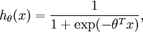
Softmax函数为多个变量的Logitic函数的泛化.
为什么使用SoftMax方法:因为反向传播和更新方法简单,更直接且直观。
1.先做练习
Exercise:Softmax Regression
Softmax regressionIn this problem set, you will use softmax regression to classify MNIST images. The goal of this exercise is to build a softmax classifier that you will be able to reuse in the future exercises and also on other classification problems that you might encounter. 在此问题集合里,你将使用SoftMax进行分类MNIST图像数据集。目标是建立一个SoftMax分类器,你将遇到其他特征练习时遇到的分类问题。 In the file softmax_exercise.zip, we have provided some starter code. You should write your code in the places indicated by "YOUR CODE HERE" in the files. In the starter code, you will need to modifysoftmaxCost.m andsoftmaxPredict.m for this exercise. We have also provided softmaxExercise.m that will help walk you through the steps in this exercise. 代码下载链接给出了一些初始预处理代码。 Dependencies 依赖项The following additional files are required for this exercise: You will also need:
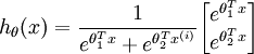
If you have not completed the exercises listed above, we strongly suggest you complete them first. Step 0: Initialize constants and parametersWe've provided the code for this step in softmaxExercise.m. 步骤一:初始化常量和参数 Two constants, inputSizeandnumClasses, corresponding to the size of each input vector and the number of class labels have been defined in the starter code. This will allow you to reuse your code on a different data set in a later exercise. We also initializelambda, the weight decay parameter here. Step 1: Load dataThe starter code loads the MNIST images and labels into inputData andlabels respectively. The images are pre-processed to scale the pixel values to the range[0,1], and the label 0 is remapped to 10 for convenience of implementation, so that the labels take values in Step 2: Implement softmaxCost - 执行软回归 代价函数In softmaxCost.m, implement code to compute the softmax cost functionJ(θ). Remember to include the weight decay term in the cost as well. Your code should also compute the appropriate gradients, as well as the predictions for the input data (which will be used in the cross-validation step later). It is important to vectorize your code so that it runs quickly. We also provide several implementation tips below: Note: In the provided starter code, theta is a matrix where each thejth row is Implementation Tip: Computing the ground truth matrix - In your code, you may need to compute the ground truth matrixM, such thatM(r, c) is 1 ify(c) =r and 0 otherwise. This can be done quickly, without a loop, using the MATLAB functionssparse andfull. Specifically, the commandM = sparse(r, c, v) creates a sparse matrix such thatM(r(i), c(i)) = v(i) for all i. That is, the vectorsr andc give the position of the elements whose values we wish to set, andv the corresponding values of the elements. Runningfull on a sparse matrix gives a "full" representation of the matrix for use (meaning that Matlab will no longer try to represent it as a sparse matrix in memory). The code for usingsparse andfull to compute the ground truth matrix has already been included in softmaxCost.m.
When the products
Hence, to prevent overflow, simply subtract some large constant value from each of the max(M) yields a row vector with each element giving the maximum value in that column.bsxfun (short for binary singleton expansion function) applies minus along each row ofM, hence subtracting the maximum of each column from every element in the column. Implementation Tip: Computing the predictions - you may also findbsxfun useful in computing your predictions - if you have a matrixM containing the The operation of bsxfun in this case is analogous to the earlier example. Step 3: Gradient checkingOnce you have written the softmax cost function, you should check your gradients numerically.In general, whenever implementing any learning algorithm, you should always check your gradients numerically before proceeding to train the model. The norm of the difference between the numerical gradient and your analytical gradient should be small, on the order of10 − 9. 一般来说,不管何时执行任何算法,你都应该 在训练模型之前 检测数值梯度? 数值距离和你的分析.计算距离 应该小于10 − 9. Implementation Tip: Faster gradient checking - when debugging, you can speed up gradient checking by reducing the number of parameters your model uses. In this case, we have included code for reducing the size of the input data, using the first 8 pixels of the images instead of the full 28x28 images. This code can be used by setting the variableDEBUG to true, as described in step 1 of the code. 快速检测:你可以归约你的参数个数。利用前8个像素而不是整个图像。 Step 4: Learning parameters--模型训练Now that you've verified that your gradients are correct, you can train your softmax model using the functionsoftmaxTraininsoftmaxTrain.m.softmaxTrain which uses the L-BFGS algorithm, in the functionminFunc. Training the model on the entire MNIST training set of 60000 28x28 images should be rather quick, and take less than 5 minutes for 100 iterations. 软回归使用L-BFGS算法,此方法在函数minFunc.里面。使用6万个图像训练,只需五分钟完成100次迭代。 Factoring softmaxTrain out as a function means that you will be able to easily reuse it to train softmax models on other data sets in the future by invoking the function with different parameters. 参数softmaxTrain 作为一个函数可使你重用软回归模型在其他数据集 仅仅是通过设置不同的参数即可以。 Use the following parameter when training your softmax classifier: Step 5: Testing-测试准确率Now that you've trained your model, you will test it against the MNIST test set, comprising 10000 28x28 images. However, to do so, you will first need to complete the functionsoftmaxPredict insoftmaxPredict.m, a function which generates predictions for input data under a trained softmax model. Once that is done, you will be able to compute the accuracy (the proportion of correctly classified images) of your model using the code provided. Our implementation achieved an accuracy of92.6%. If your model's accuracy is significantly less (less than 91%), check your code, ensure that you are using the trained weights, and that you are training your model on the full 60000 training images. Conversely, if your accuracy is too high (99-100%), ensure that you have not accidentally trained your model on the test set as well. 利用预测函数softmaxPredict.m检测准确率。 |
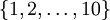 . You will not need to change any code in this step for this exercise, but note that your code should be general enough to operate on data of arbitrary size belonging to any number of classes.
 are large, the exponential function
 will become very large and possibly overflow. When this happens, you will not be able to compute your hypothesis. However, there is an easy solution - observe that we can multiply the top and bottom of the hypothesis by some constant without changing the output:
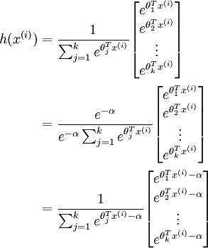
 terms before computing the exponential. In practice, for each example, you can use the maximum of the
 , then you can use the following code to accomplish this:
 terms, such thatM(r, c) contains the
 term, you can use the following code to compute the hypothesis (by dividing all elements in each column by their column sum):
2.解析模型---Softmax Regression
Contents[hide] |
Introduction
In these notes, we describe theSoftmax regression model. This model generalizes logistic regression toclassification problems where the class labely can take on more than two possible values.This will be useful for such problems as MNIST digit classification, where the goal is to distinguish between 10 differentnumerical digits. Softmax regression is a supervised learning algorithm, but we will later beusing it in conjuction with our deep learning/unsupervised feature learning methods.
软回归是逻辑斯特递归模型延伸的多类分类器。
Recall that in logistic regression, we had a training set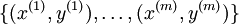 ofm labeled examples, where the input features are
 . (In this set of notes, we will use the notational convention of letting the feature vectorsx ben + 1 dimensional, withx0 = 1 corresponding to the intercept term.) With logistic regression, we were in the binary classification setting, so the labels were
 . Our hypothesis took the form:
 ( 对于二分类的要求,目标函数为,我们使用Sigmod函数,模型参数θ去训练最小化代价函数)
and the model parameters θ were trained to minimizethe cost function
![\begin{align}J(\theta) = -\frac{1}{m} \left[ \sum_{i=1}^m y^{(i)} \log h_\theta(x^{(i)}) + (1-y^{(i)}) \log (1-h_\theta(x^{(i)})) \right]\end{align}](http://deeplearning.stanford.edu/wiki/images/math/f/a/6/fa6565f1e7b91831e306ec404ccc1156.png)
In the softmax regression setting, we are interested in multi-classclassification (as opposed to only binary classification), and so the labely can take onk different values,rather than only two. Thus, in our training set,we now have that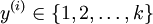 . (Note thatour convention will be to index the classes starting from 1, rather than from 0.) For example,in the MNIST digit recognition task, we would havek = 10 different classes.
( 多类分类的目标函数为。)
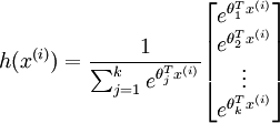
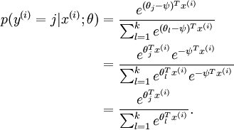
Given a test input x, we want our hypothesis to estimatethe probability thatp(y =j |x) for each value of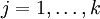 .I.e., we want to estimate the probability of the class label taking on each of thek different possible values. Thus, our hypothesis will output ak dimensional vector (whose elements sum to 1) giving us ourk estimated probabilities. Concretely, our hypothesishθ(x) takes the form:
(由此,我们假设 k 维向量(元素和为1)表示我们的k个特征的估值概率。形式如下:)
Here 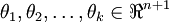 are the parameters of our model. Notice that the term
 normalizes the distribution, so that it sums to one.
For convenience, we will also write θ to denote all the parameters of our model. When you implement softmax regression, it is usually convenient to representθ as ak-by-(n + 1) matrix obtained by stacking up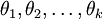 in rows, so that
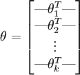 ( 即时我们的模型参数,列向量的表示应该是比较方便的。)
Cost Function-估价函数
We now describe the cost function that we'll use for softmax regression. In the equation below, istheindicator function, so that 1{a true statement} = 1, and1{a false statement} = 0.For example,1{2 + 2 = 4} evaluates to 1; whereas1{1 + 1 = 5} evaluates to 0. Our cost function will be:
![\begin{align}J(\theta) = - \frac{1}{m} \left[ \sum_{i=1}^{m} \sum_{j=1}^{k} 1\left\{y^{(i)} = j\right\} \log \frac{e^{\theta_j^T x^{(i)}}}{\sum_{l=1}^k e^{ \theta_l^T x^{(i)} }}\right]\end{align}](http://deeplearning.stanford.edu/wiki/images/math/7/6/3/7634eb3b08dc003aa4591a95824d4fbd.png)
Notice that this generalizes the logistic regression cost function, which could also have been written:
![\begin{align}J(\theta) &= -\frac{1}{m} \left[ \sum_{i=1}^m (1-y^{(i)}) \log (1-h_\theta(x^{(i)})) + y^{(i)} \log h_\theta(x^{(i)}) \right] \\&= - \frac{1}{m} \left[ \sum_{i=1}^{m} \sum_{j=0}^{1} 1\left\{y^{(i)} = j\right\} \log p(y^{(i)} = j | x^{(i)} ; \theta) \right]\end{align}](http://deeplearning.stanford.edu/wiki/images/math/5/4/9/5491271f19161f8ea6a6b2a82c83fc3a.png)
The softmax cost function is similar, except that we now sum over thek different possible valuesof the class label. Note also that in softmax regression, we have that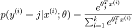 .
.
There is no known closed-form way to solve for the minimum ofJ(θ), and thus as usual we'll resort to an iterativeoptimization algorithm such as gradient descent or L-BFGS. Taking derivatives, one can show that the gradient is:
![\begin{align}\nabla_{\theta_j} J(\theta) = - \frac{1}{m} \sum_{i=1}^{m}{ \left[ x^{(i)} \left( 1\{ y^{(i)} = j\} - p(y^{(i)} = j | x^{(i)}; \theta) \right) \right] }\end{align}](http://deeplearning.stanford.edu/wiki/images/math/5/9/e/59ef406cef112eb75e54808b560587c9.png)
Recall the meaning of the " " notation. In particular,
 is itself a vector, so that itsl-th element is
 the partial derivative ofJ(θ) with respect to thel-th element ofθj. ( 本身是一个向量,对其求偏导数)
Armed with this formula for the derivative, one can then plug it into an algorithm such as gradient descent, and have itminimizeJ(θ). For example, with the standard implementation of gradient descent, on each iterationwe would perform the update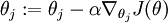 (for each).
When implementing softmax regression, we will typically use a modified version of the cost function described above;specifically, one that incorporates weight decay. We describe the motivation and details below.
Properties of softmax regression parameterization
Softmax regression has an unusual property that it has a "redundant" set of parameters. To explain what this means, suppose we take each of our parameter vectorsθj, and subtract some fixed vectorψfrom it, so that everyθj is now replaced withθj − ψ (for every). Our hypothesis now estimates the class label probabilities as
(软回归有“过多的”参数集合,即过参数化了,意味着对于我们想要拟合数据集的假设,超过了需要拟合假设的一般量的参数个数)
In other words, subtracting ψ from every θjdoes not affect our hypothesis' predictions at all! This shows that softmaxregression's parameters are "redundant." More formally, we say that oursoftmax model isoverparameterized, meaning that for any hypothesis we might fit to the data, there are multiple parameter settings that give rise to exactly the same hypothesis functionhθ mapping from inputsxto the predictions.
Further, if the cost function J(θ) is minimized by somesetting of the parameters ,then it is also minimized by
 for any value ofψ. Thus, theminimizer of J(θ) is not unique. (Interestingly,J(θ) is still convex, and thus gradient descent willnot run into a local optima problems. But the Hessian is singular/non-invertible,which causes a straightforward implementation of Newton's method to run intonumerical problems.)
()
Notice also that by setting ψ = θ1, one can alwaysreplaceθ1 with (the vector of all0's), without affecting the hypothesis. Thus, one could "eliminate" the vectorof parametersθ1 (or any otherθj, forany single value ofj), without harming the representational powerof our hypothesis. Indeed, rather than optimizing over thek(n + 1)parameters (where
 ), one could instead set
 and optimize only with respect to the(k − 1)(n + 1)remaining parameters, and this would work fine.
In practice, however, it is often cleaner and simpler to implement the version which keepsall the parameters , withoutarbitrarily setting one of them to zero. But we willmake one change to the cost function: Adding weight decay. This will take care ofthe numerical problems associated with softmax regression's overparameterized representation.
Weight Decay
We will modify the cost function by adding a weight decay term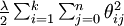 which penalizes large values of the parameters. Our cost function is now
![\begin{align}J(\theta) = - \frac{1}{m} \left[ \sum_{i=1}^{m} \sum_{j=1}^{k} 1\left\{y^{(i)} = j\right\} \log \frac{e^{\theta_j^T x^{(i)}}}{\sum_{l=1}^k e^{ \theta_l^T x^{(i)} }} \right] + \frac{\lambda}{2} \sum_{i=1}^k \sum_{j=0}^n \theta_{ij}^2\end{align}](http://deeplearning.stanford.edu/wiki/images/math/4/7/1/471592d82c7f51526bb3876c6b0f868d.png)
With this weight decay term (for anyλ > 0), the cost functionJ(θ) is now strictly convex, and is guaranteed to have aunique solution. The Hessian is now invertible, and becauseJ(θ) is convex, algorithms such as gradient descent, L-BFGS, etc. are guaranteedto converge to the global minimum.
To apply an optimization algorithm, we also need the derivative of thisnew definition ofJ(θ). One can show that the derivative is:![\begin{align}\nabla_{\theta_j} J(\theta) = - \frac{1}{m} \sum_{i=1}^{m}{ \left[ x^{(i)} ( 1\{ y^{(i)} = j\} - p(y^{(i)} = j | x^{(i)}; \theta) ) \right] } + \lambda \theta_j\end{align}](http://deeplearning.stanford.edu/wiki/images/math/3/a/f/3afb4b9181a3063ddc639099bc919197.png)
By minimizing J(θ) with respect to θ, we will have a working implementation of softmax regression.
Relationship to Logistic Regression-和逻辑递归的关系
In the special case where k = 2, one can show that softmax regression reduces to logistic regression.This shows that softmax regression is a generalization of logistic regression. Concretely, whenk = 2,the softmax regression hypothesis outputs
Taking advantage of the fact that this hypothesisis overparameterized and settingψ = θ1,we can subtractθ1 from each of the two parameters, giving us
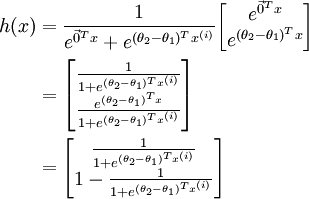
Thus, replacing θ2 − θ1 with a single parameter vectorθ', we findthat softmax regression predicts the probability of one of the classes as ,and that of the other class as
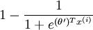 ,same as logistic regression.
Softmax Regression vs. k Binary Classifiers--和k个二分类器的比较
Suppose you are working on a music classification application, and there arek types of music that you are trying to recognize. Should you use asoftmax classifier, or should you buildk separate binary classifiers usinglogistic regression?
This will depend on whether the four classes aremutually exclusive. For example,if your four classes are classical, country, rock, and jazz, then assuming eachof your training examples is labeled with exactly one of these four class labels,you should build a softmax classifier withk = 4.(If there're also some examples that are none of the above four classes,then you can setk = 5 in softmax regression, and also have a fifth, "none of the above," class.)
If however your categories are has_vocals, dance, soundtrack, pop, then theclasses are not mutually exclusive; for example, there can be a piece of popmusic that comes from a soundtrack and in addition has vocals. In this case, itwould be more appropriate to build 4 binary logistic regression classifiers. This way, for each new musical piece, your algorithm can separately decide whetherit falls into each of the four categories.
Now, consider a computer vision example, where you're trying to classify images intothree different classes. (i) Suppose that your classes are indoor_scene , outdoor_urban_scene, and outdoor_wilderness_scene. Would you use sofmax regressionor three logistic regression classifiers? (ii) Now suppose your classes areindoor_scene, black_and_white_image, and image_has_people. Would you use softmaxregression or multiple logistic regression classifiers?
In the first case, the classes are mutually exclusive, so a softmax regressionclassifier would be appropriate. In the second case, it would be more appropriate to buildthree separate logistic regression classifiers.
对于多类分类问题,是建立一个 软回归分类器还是建立多个二分类器呢?
这依赖于你的多类是否互斥,软回归 分类器对集合的分类是划分而不是覆盖。
...................
考虑一个计算机视觉的问题,如果你对图像分类 ,类别是 室内、室外市区、室外草地场景,你将使用软回归还是三个二分类器?若类别是室外场景、黑白图像、有人的图像,又将使用哪种方式?
答案是 第一种分类使用软回归,第二种分类使用多个二分类器,因为第一个类别集合是划分,而第二个类别集合有覆盖。
3.另外一个翻译
原文链接:http://blog.csdn.net/celerychen2009/article/details/9014797
. 对开源softmax回归的一点解释
对深度学习的开源代码中有一段softmax的代码,下载链接如下:
https://github.com/yusugomori/DeepLearning
这个开源的代码是实现了深度网络的常见算法,包括c,c++,java,python等不同语言的版本。
softmax回归中有这样一段代码:
void LogisticRegression_softmax(LogisticRegression *this, double *x)
{
  int i;
  double max = 0.0;
  double sum = 0.0;

  for(i=0; i<this->n_out; i++) if(max < x[i]) max = x[i];

  for(i=0; i<this->n_out; i++) {
    x[i] = <span style="color:#000099;">exp</span>(x[i] - max);
    sum += x[i];
  }

  for(i=0; i<this->n_out; i++) x[i] /= sum;
}Tips:乍一看这段代码,发现它和文献中对softmax模型中参数优化的迭代公式中是不一样!其实,如果没有那个求最大值的过程,直接取指数运算就一样的。而加一个求最大值的好处在于避免数据的绝对值过小,数据绝对值太小可能会导致计算一直停留在零而无法进行。就像对数似然函数,似然函数取对数防止概率过小一样。
从新翻译没有多大意义!


 1178
1178


 被折叠的 条评论
为什么被折叠?
被折叠的 条评论
为什么被折叠?
 到【灌水乐园】发言


