


1.欧几里得距离
Euclidean distance 欧氏距离也称欧几里得距离,它是一个通常采用的距离定义,它是在m维空间中两个点之间的真实距离。
二维的公式
三维的公式
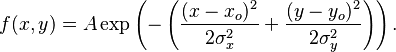
欧氏距离的公式
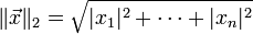
欧几里得度量定义欧几里得空间中,点 x = ( x 1,..., x n) 和 y = ( y 1,..., y n) 之间的距离为
-

-
向量
 的自然长度,即该点到原点的距离为
-
 .
.
它是一个纯数值。在欧几里得度量下,两点之间直线最短。
2.拉格朗日插值法
http://zh.wikipedia.org/wiki/%E6%8B%89%E6%A0%BC%E6%9C%97%E6%97%A5%E6%8F%92%E5%80%BC%E6%B3%95
3.景深效果 Depth of field
http://en.wikipedia.org/wiki/Depth_of_field
4.多普勒效应(声音)
http://zh.wikipedia.org/wiki/%E5%A4%9A%E6%99%AE%E5%8B%92%E6%95%88%E5%BA%94
公式
观察者 (Observer) 和发射源 (Source) 的频率关系为: 
 为观察到的频率;
 为发射源于该介质中的原始发射频率;
 为波在该介质中的行进速度;
 为观察者相对于介质的移动速度,若接近发射源则前方运算符号为 + 号`, 反之则为 - 号;
 为发射源相对于介质的移动速度,若接近观察者则前方运算符号为 - 号,反之则为 + 号。
5.拓扑学(拓扑结构)
http://baike.baidu.com/view/41881.htm?fr=aladdin
6.点积(数量积,无向积)
两个向量a = [a1, a2,…, an]和b = [b1, b2,…, bn]的点积定义为
a·b=a1b1+a2b2+……+anbn
http://baike.baidu.com/view/2744555.htm?fr=aladdin
7.叉积(向量积,矢量积)
http://baike.baidu.com/item/%E5%90%91%E9%87%8F%E7%A7%AF?from_id=2812058&type=syn&fromtitle=%E5%8F%89%E7%A7%AF&fr=aladdin
8.哈希算法
常用字符串哈希函数有 BKDRHash,APHash,DJBHash,JSHash,RSHash,SDBMHash,PJWHash,ELFHash等等。对于以上几种哈希函数,对其进行了一个小小的评测。
| Hash函数 | 数据1 | 数据2 | 数据3 | 数据4 | 数据1得分 | 数据2得分 | 数据3得分 | 数据4得分 | 平均分 |
| BKDRHash | 2 | 0 | 4774 | 481 | 96.55 | 100 | 90.95 | 82.05 | 92.64 |
| APHash | 2 | 3 | 4754 | 493 | 96.55 | 88.46 | 100 | 51.28 | 86.28 |
| DJBHash | 2 | 2 | 4975 | 474 | 96.55 | 92.31 | 0 | 100 | 83.43 |
| JSHash | 1 | 4 | 4761 | 506 | 100 | 84.62 | 96.83 | 17.95 | 81.94 |
| RSHash | 1 | 0 | 4861 | 505 | 100 | 100 | 51.58 | 20.51 | 75.96 |
| SDBMHash | 3 | 2 | 4849 | 504 | 93.1 | 92.31 | 57.01 | 23.08 | 72.41 |
| PJWHash | 30 | 26 | 4878 | 513 | 0 | 0 | 43.89 | 0 | 21.95 |
| ELFHash | 30 | 26 | 4878 | 513 | 0 | 0 | 43.89 | 0 | 21.95 |
http://baike.baidu.com/view/273836.htm?fr=aladdin
ELFHash
http://blog.csdn.net/yinxusen/article/details/6317466
BKDRHash
http://www.360doc.com/content/14/0610/10/14505022_385328710.shtml
9.哈希表
http://baike.baidu.com/view/329976.htm?fr=aladdin
http://blog.chinaunix.net/uid-24951403-id-2212565.html
unity3d 哈希表
http://www.tuicool.com/articles/ABzUFjf
10.最小二乘法
http://baike.baidu.com/link?url=M6K_E5mDVXU9Yn7COxW2fs-V5viOTgnpuMDiTahj_oFX0bmFbqss0OFjBkMvyEvMFAZnqR1VWBG8bf5jpZAfoa
11.Poisson Disc
float3 SiGrowablePoissonDisc13FilterRGB
(sampler tSource, float2 texCoord, float2 pixelSize, float discRadius)
{
float3 cOut;
float2 poisson[12] = {float2(-0.326212f, -0.40581f),
float2(-0.840144f, -0.07358f),
float2(-0.695914f, 0.457137f),
float2(-0.203345f, 0.620716f),
float2(0.96234f, -0.194983f),
float2(0.473434f, -0.480026f),
float2(0.519456f, 0.767022f),
float2(0.185461f, -0.893124f),
float2(0.507431f, 0.064425f),
float2(0.89642f, 0.412458f),
float2(-0.32194f, -0.932615f),
float2(-0.791559f, -0.59771f)};
// Center tap
cOut = tex2D (tSource, texCoord);
for (int tap = 0; tap < 12; tap++)
{
float2 coord = texCoord.xy + (pixelSize * poisson[tap] * discRadius);
// Sample pixel
cOut += tex2D (tSource, coord);
}
return (cOut / 13.0f);
}
12.Gaussian function
http://en.wikipedia.org/wiki/Gaussian_function
wiki
In mathematics, a Gaussian function, often simply referred to as aGaussian, is afunction of the form:

for arbitrary real constants a, b and c. It is named after the mathematicianCarl Friedrich Gauss.
The graph of a Gaussian is a characteristic symmetric "bell curve" shape. The parametera is the height of the curve's peak, b is the position of the center of the peak andc (thestandard deviation, sometimes called the Gaussian RMS width) controls the width of the "bell".
Gaussian functions are widely used in statistics where they describe the normal distributions, in signal processing where they serve to define Gaussian filters, in image processing where two-dimensional Gaussians are used for Gaussian blurs, and in mathematics where they are used to solve heat equations and diffusion equations and to define the Weierstrass transform.
Properties
Gaussian functions arise by composing the exponential function with a concave quadratic function. The Gaussian functions are thus those functions whose logarithm is a concave quadratic function.
The parameter c is related to the full width at half maximum (FWHM) of the peak according to

Alternatively, the parameter c can be interpreted by saying that the twoinflection points of the function occur at x = b − c andx = b + c.
The full width at tenth of maximum (FWTM) for a Gaussian could be of interest and is

Gaussian functions are analytic, and their limit as x → ∞ is 0 (for the above case ofd = 0).
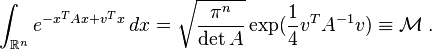
Gaussian functions are among those functions that are elementary but lack elementary antiderivatives; the integral of the Gaussian function is the error function. Nonetheless their improper integrals over the whole real line can be evaluated exactly, using theGaussian integral
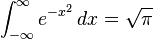
and one obtains
This integral is 1 if and only if  , and in this case the Gaussian is theprobability density function of a normally distributed random variable with expected value μ = b and variance σ2 = c2:
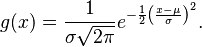
These Gaussians are plotted in the accompanying figure.
Gaussian functions centered at zero minimize the Fourier uncertainty principle.
The product of two Gaussian functions is a Gaussian, and the convolution of two Gaussian functions is also a Gaussian, with variance being the sum of the original variances: . The product of two Gaussian probability density functions, though, is not in general a Gaussian PDF.
Taking the Fourier transform (unitary, angular frequency convention) of a Gaussian function with parametersa = 1,b = 0 andc yields another Gaussian function, with parameters ,b = 0 and
 .[3] So in particular the Gaussian functions with b = 0 and
 are kept fixed by the Fourier transform (they areeigenfunctions of the Fourier transform with eigenvalue 1). A physical realization is that of thediffraction pattern: for example, a photographic slide whose transmissivity has a Gaussian variation is also a Gaussian function.
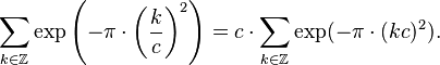
The fact that the Gaussian function is an eigenfunction of the continuous Fourier transform allows us to derive the following interesting identity from thePoisson summation formula:
Integral of a Gaussian function
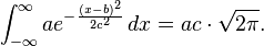
The integral of an arbitrary Gaussian function is
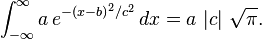
An alternative form is

where f must be strictly positive for the integral to converge.
Proof
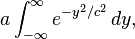
The integral

for some real constants a, b, c > 0 can be calculated by putting it into the form of aGaussian integral. First, the constanta can simply be factored out of the integral. Next, the variable of integration is changed fromx toy = x + b.
and then to 

Then, using the Gaussian integral identity
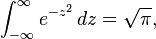
we have

Two-dimensional Gaussian function

In two dimensions, the power to which e is raised in the Gaussian function is any negative-definite quadratic form. Consequently, the level sets of the Gaussian will always be ellipses.
A particular example of a two-dimensional Gaussian function is
Here the coefficient A is the amplitude, xo,yo is the center and σx, σy are thex andy spreads of the blob. The figure on the right was created usingA = 1,xo = 0, yo = 0, σx = σy = 1.
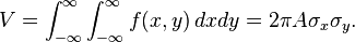
The volume under the Gaussian function is given by
In general, a two-dimensional elliptical Gaussian function is expressed as

where the matrix
![\left[\begin{matrix} a & b \\ b & c \end{matrix}\right]](http://upload.wikimedia.org/math/5/3/f/53f022c87448b5afdf1062ec965f4db7.png)
Using this formulation, the figure on the right can be created using A = 1, (xo,yo) = (0, 0),a =c = 1/2,b = 0.
Meaning of parameters for the general equation
For the general form of the equation the coefficient A is the height of the peak and (xo, yo) is the center of the blob.
If we set
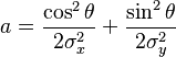

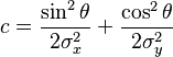
then we rotate the blob by a clockwise angle  (for counterclockwise rotation invert the signs in the b coefficient). This can be seen in the following examples:

|

|

|

|

|

|
Using the following Octave code one can easily see the effect of changing the parameters
A = 1;
x0 = 0; y0 = 0;

sigma_x = 1;
sigma_y = 2;

[X, Y] = meshgrid(-5:.1:5, -5:.1:5);

for theta = 0:pi/100:pi
    a = cos(theta)^2/2/sigma_x^2 + sin(theta)^2/2/sigma_y^2;
    b = -sin(2*theta)/4/sigma_x^2 + sin(2*theta)/4/sigma_y^2 ;
    c = sin(theta)^2/2/sigma_x^2 + cos(theta)^2/2/sigma_y^2;

    Z = A*exp( - (a*(X-x0).^2 + 2*b*(X-x0).*(Y-y0) + c*(Y-y0).^2)) ;
end

surf(X,Y,Z);shading interp;view(-36,36)
Such functions are often used in image processing and in computational models of visual system function—see the articles on scale space and affine shape adaptation.
Also see multivariate normal distribution.
Multi-dimensional Gaussian function
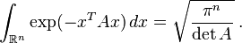
In an  -dimensional space a Gaussian function can be defined as
where 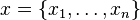 is a column of coordinates,
 is apositive-definite
 matrix, and
 denotestransposition.
The integral of this Gaussian function over the whole -dimensional space is given as
It can be easily calculated by diagonalizing the matrix and changing the integration variables to the eigenvectors of .
More generally a shifted Gaussian function is defined as

where 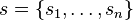 is the shift vector and the matrix can be assumed to be symmetric,
 , and positive-definite. The following integrals with this function can be calculated with the same technique,


Gaussian profile estimation
A number of fields such as stellar photometry, Gaussian beam characterization, and emission/absorption line spectroscopy work with sampled Gaussian functions and need to accurately estimate the height, position, and width parameters of the function. These are ,
, , and
, and for a 1D Gaussian function,,
 , and
, and for a 2D Gaussian function. The most common method for estimating the profile parameters is to take the logarithm of the data and fit a parabola to the resulting data set.[4] While this provides a simple least squares fitting procedure, the resulting algorithm is biased by excessively weighting small data values, and this can produce large errors in the profile estimate. One can partially compensate for this throughweighted least squares estimation, in which the small data values are given small weights, but this too can be biased by allowing the tail of the Gaussian to dominate the fit. In order to remove the bias, one can instead use an iterative procedure in which the weights are updated at each iteration (see Iteratively reweighted least squares).[4]
Once one has an algorithm for estimating the Gaussian function parameters, it is also important to know how accurate those estimates are. While an estimation algorithm can provide numerical estimates for the variance of each parameter (i.e. the variance of the estimated height, position, and width of the function), one can use Cramér–Rao bound theory to obtain an analytical expression for the lower bound on the parameter variances, given some assumptions about the data.[5][6]
- The noise in the measured profile is either i.i.d. Gaussian, or the noise is Poisson-distributed.
- The spacing between each sampling (i.e. the distance between pixels measuring the data) is uniform.
- The peak is "well-sampled", so that less than 10% of the area or volume under the peak (area if a 1D Gaussian, volume if a 2D Gaussian) lies outside the measurement region.
- The width of the peak is much larger than the distance between sample locations (i.e. the detector pixels must be at least 5 times smaller than the Gaussian FWHM).
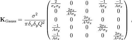
When these assumptions are satisfied, the following covariance matrix K applies for the 1D profile parameters ,, and under i.i.d. Gaussian noise and under Poisson noise:[5]

where  is the width of the pixels used to sample the function,
 is the quantum efficiency of the detector, and
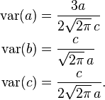
 indicates the standard deviation of the measurement noise. Thus, the individual variances for the parameters are, in the Gaussian noise case,
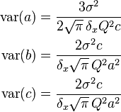
and in the Poisson noise case,
For the 2D profile parameters giving the amplitude , position, and width of the profile, the following covariance matrices apply:[6]

where the individual parameter variances are given by the diagonal elements of the covariance matrix.
Discrete Gaussian

One may ask for a discrete analog to the Gaussian; this is necessary in discrete applications, particularlydigital signal processing. A simple answer is to sample the continuous Gaussian, yielding thesampled Gaussian kernel. However, this discrete function does not have the discrete analogs of the properties of the continuous function, and can lead to undesired effects, as described in the articlescale space implementation.
An alternative approach is to use discrete Gaussian kernel:[7]
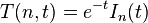
where  denotes themodified Bessel functions of integer order.
This is the discrete analog of the continuous Gaussian in that it is the solution to the discretediffusion equation (discrete space, continuous time), just as the continuous Gaussian is the solution to the continuous diffusion equation.[8]
12.一个随机数算法
<span style="font-size:14px;">float scale = 0.5;
float magic = 3571.0;float2 random = ( 1.0 / 4320.0 ) * position +	float2( 0.25, 0.0 );random = frac( dot( random * random, magic ) );
random = frac( dot( random * random, magic ) );
return -scale + 2.0 * scale * random;</span>

13.一个棋盘算法
in unity
<span style="font-size:14px;">				float scale = 0.25;
				float2 positionMod = float2(uint2(i.uv_MainTex*10) & 1);
				return (-scale + 2.0 * scale * positionMod.x) *
					(-1.0 + 2.0 * positionMod.y);
</span>
float scale = 0.25;
float2 positionMod = float2(uint2(i.uv_MainTex*10) & 1);
return (-scale + 2.0 * scale * positionMod.x) *
(-1.0 + 2.0 * positionMod.y) +
0.5 * scale * (-1.0 + 2.0 * _frameCountMod);//<span style="font-size:14px;"></span><pre name="code" class="cpp">//_frameCountMod参数实现对棋盘的控制<span style="font-size:14px;">float scale = 0.25;
float2 positionMod = float2( uint2( sv_position ) & 1 );
return ( -scale + 2.0 * scale * positionMod.x ) *
( -1.0 + 2.0 * positionMod.y );
</span>

14.kNN(K-Nearest Neighbor)最邻近规则分类
http://blog.csdn.net/xlm289348/article/details/8876353
KNN最邻近规则,主要应用领域是对未知事物的识别,即判断未知事物属于哪一类,判断思想是,基于欧几里得定理,判断未知事物的特征和哪一类已知事物的的特征最接近;
K最近邻(k-Nearest Neighbor,KNN)分类算法,是一个理论上比较成熟的方法,也是最简单的机器学习算法之一。该方法的思路是:如果一个样本在特征空间中的k个最相似(即特征空间中最邻近)的样本中的大多数属于某一个类别,则该样本也属于这个类别。KNN算法中,所选择的邻居都是已经正确分类的对象。该方法在定类决策上只依据最邻近的一个或者几个样本的类别来决定待分样本所属的类别。 KNN方法虽然从原理上也依赖于极限定理,但在类别决策时,只与极少量的相邻样本有关。由于KNN方法主要靠周围有限的邻近的样本,而不是靠判别类域的方法来确定所属类别的,因此对于类域的交叉或重叠较多的待分样本集来说,KNN方法较其他方法更为适合。
KNN算法不仅可以用于分类,还可以用于回归。通过找出一个样本的k个最近邻居,将这些邻居的属性的平均值赋给该样本,就可以得到该样本的属性。更有用的方法是将不同距离的邻居对该样本产生的影响给予不同的权值(weight),如权值与距离成正比(组合函数)。
该算法在分类时有个主要的不足是,当样本不平衡时,如一个类的样本容量很大,而其他类样本容量很小时,有可能导致当输入一个新样本时,该样本的K个邻居中大容量类的样本占多数。 该算法只计算“最近的”邻居样本,某一类的样本数量很大,那么或者这类样本并不接近目标样本,或者这类样本很靠近目标样本。无论怎样,数量并不能影响运行结果。可以采用权值的方法(和该样本距离小的邻居权值大)来改进。该方法的另一个不足之处是计算量较大,因为对每一个待分类的文本都要计算它到全体已知样本的距离,才能求得它的K个最近邻点。目前常用的解决方法是事先对已知样本点进行剪辑,事先去除对分类作用不大的样本。该算法比较适用于样本容量比较大的类域的自动分类,而那些样本容量较小的类域采用这种算法比较容易产生误分。
K-NN可以说是一种最直接的用来分类未知数据的方法。基本通过下面这张图跟文字说明就可以明白K-NN是干什么的

简单来说,K-NN可以看成:有那么一堆你已经知道分类的数据,然后当一个新数据进入的时候,就开始跟训练数据里的每个点求距离,然后挑离这个训练数据最近的K个点看看这几个点属于什么类型,然后用少数服从多数的原则,给新数据归类。
算法步骤:
step.1---初始化距离为最大值
step.2---计算未知样本和每个训练样本的距离dist
step.3---得到目前K个最临近样本中的最大距离maxdist
step.4---如果dist小于maxdist,则将该训练样本作为K-最近邻样本
step.5---重复步骤2、3、4,直到未知样本和所有训练样本的距离都算完
step.6---统计K-最近邻样本中每个类标号出现的次数
step.7---选择出现频率最大的类标号作为未知样本的类标号
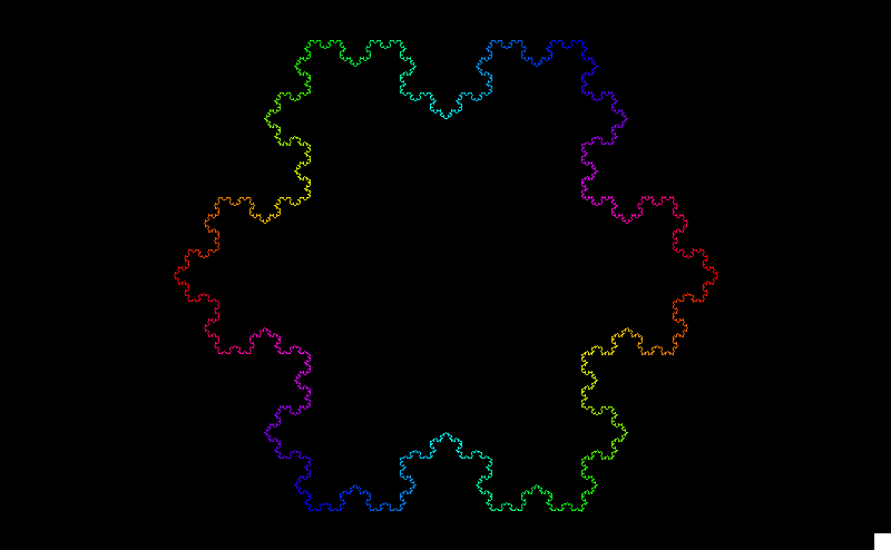
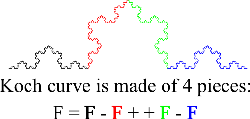
15.科赫曲线Koch Curve
科赫曲线是一种像雪花的几何曲线,所以又称为雪花曲线,它是de Rham曲线的特例。
15.误差函数
在数学中,误差函数(也称之为
高斯误差函数,error function or Gauss error function)是一个非基本函数(即不是
初等函数),其在
概率论、统计学以及偏
微分方程,半导体物理中都有广泛地应用。
定义


导数与积分


级数展开式


 9857
9857

 被折叠的 条评论
为什么被折叠?
被折叠的 条评论
为什么被折叠?
 到【灌水乐园】发言


