主成分分析（PCA）-理论基础

转载 http://www.cnblogs.com/jerrylead

要解释为什么协方差矩阵的特征向量可以将原始特征映射到 k 维理想特征，我看到的有三个理论：分别是最大方差理论、最小错误理论和坐标轴相关度理论。这里简单探讨前两种，最后一种在讨论PCA 意义时简单概述。

最大方差理论

在信号处理中认为信号具有较大的方差，噪声有较小的方差，信噪比就是信号与噪声的方差比，越大越好。如前面的图，样本在横轴上的投影方差较大，在纵轴上的投影方差较小，那么认为纵轴上的投影是由噪声引起的。

因此我们认为，最好的 k 维特征是将 n 维样本点转换为 k 维后，每一维上的样本方差都很大。

比如下图有 5 个样本点：（已经做过预处理，均值为 0，特征方差归一）

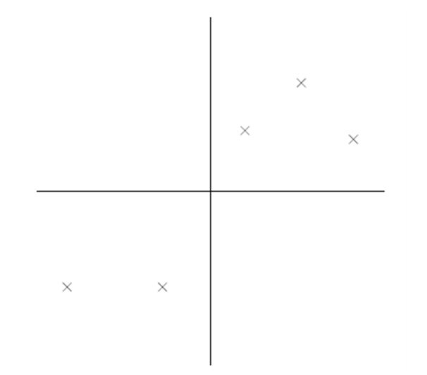
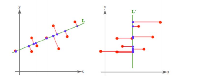
下面将样本投影到某一维上，这里用一条过原点的直线表示（之前预处理的过程实质是将原点移到样本点的中心点）。

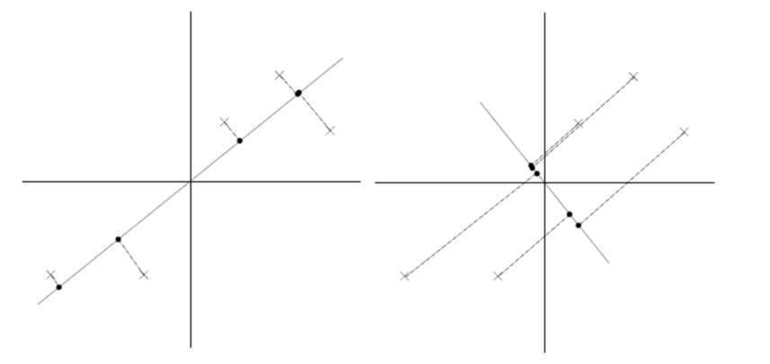
假设我们选择两条不同的直线做投影，那么左右两条中哪个好呢？根据我们之前的方差最大化理论，左边的好，因为投影后的样本点之间方差最大。

这里先解释一下投影的概念：

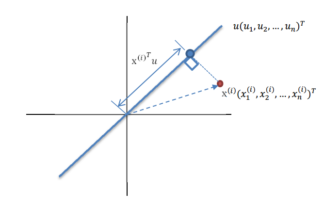
红色点表示样例$x^{(i)}$,蓝色点表示$x^{(i)}$在$u$上的投影，$u$是直线的斜率也是直线的方向向量，而且是单位向量。蓝色点是$x^{(i)}$在$u$上的投影点，离原点的距离是$<x^{(i)},u>（即{x^{(i)}}^Tu或u^Tx{(i)}）$由于这些样本点（样例）的每一维特征均值都为 0，因此投影到 u 上的样本点（只有一个到原点的距离值）的均值仍然是 0。

回到上面左右图中的左图，我们要求的是最佳的 u，使得投影后的样本点方差最大。

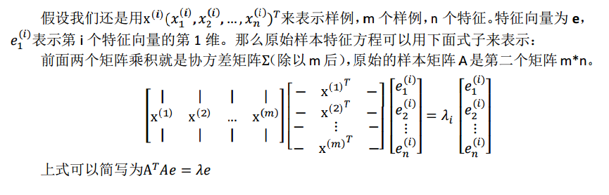
由于投影后均值为 0，因此方差为：

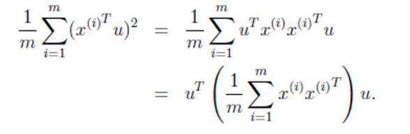
中间那部分很熟悉啊，不就是样本特征的协方差矩阵么($x^{(i)}$的均值为 0，一般协方差矩阵都除以 m‐1，这里用 m）。

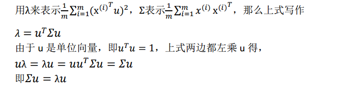
We got it！λ就是Σ的特征值，u 是特征向量。最佳的投影直线是特征值λ最大时对应的特征向量，其次是λ第二大对应的特征向量，依次类推。

因此，我们只需要对协方差矩阵进行特征值分解，得到的前 k 大特征值对应的特征向量就是最佳的 k 维新特征，而且这 k 维新特征是正交的。得到前 k 个 u 以后，样例$x^{(i)}$通过以下变换可以得到新的样本:

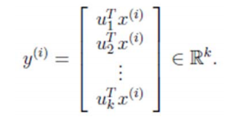
通过选取最大的 k 个 u，使得方差较小的特征（如噪声）被丢弃。
这是其中一种对 PCA 的解释，第二种是错误最小化。

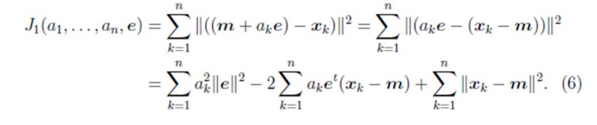
最小平方误差理论

假设有这样的二维样本点（红色点），回顾我们前面探讨的是求一条直线，使得样本点投影到直线上的点的方差最大。本质是求直线，那么度量直线求的好不好，不仅仅只有方差最大化的方法。再回想我们最开始学习的线性回归等，目的也是求一个线性函数使得直线能够最佳拟合样本点，那么我们能不能认为最佳的直线就是回归后的直线呢？回归时我们的最小二乘法度量的是样本点到直线的坐标轴距离。比如这个问题中，特征是 x，类标签是 y。回归时最小二乘法度量的是距离 d。如果使用回归方法来度量最佳直线，那么就是直接在原始样本上做回归了，跟特征选择就没什么关系了。

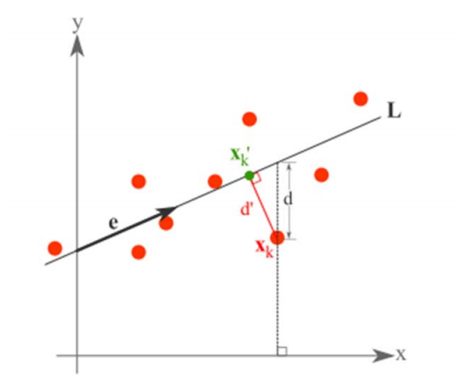
因此，我们打算选用另外一种评价直线好坏的方法，使用点到直线的距离 d’来度量。
现在有 n 个样本点($x_1,...,x_n$)，每个样本点为 m 维（这节内容中使用的符号与上面的不太一致，需要重新理解符号的意义）。将样本点$x_k$在直线上的投影记为$x_k'$，那么我们就是要最小化

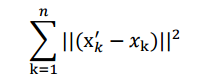
这个公式称作最小平方误差（Least Squared Error）。
而确定一条直线，一般只需要确定一个点以及方向即可。

第一步确定点：

假设要在空间中找一点$x_0$来代表这 n 个样本点，“代表”这个词不是量化的，因此要量化成，我们就是要找一个 m 维的点$x_0$，使得:

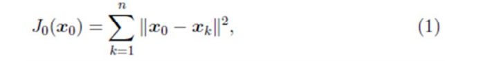
最小。其中$J_0(x_0)$是平方错误评价函数（squared‐error criterion function），假设 m 为 n个样本点的均值：

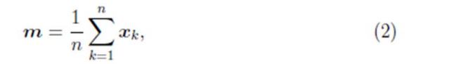
那么平方错误可以写作：

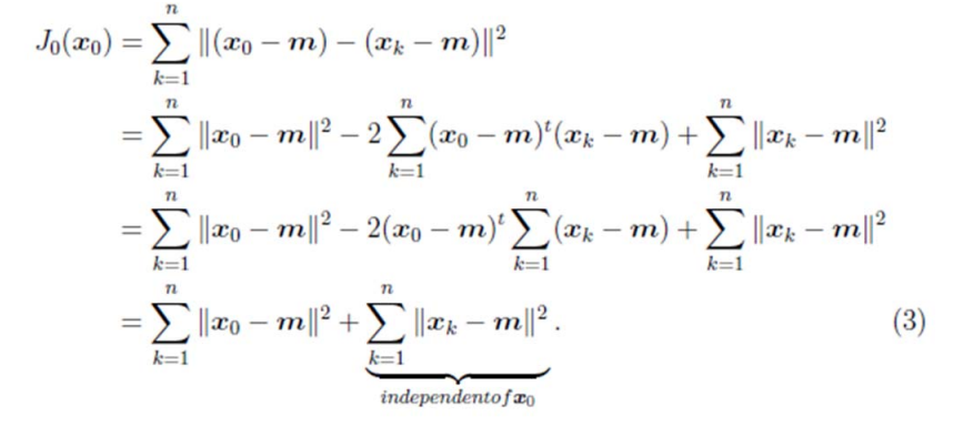
第一行就类似坐标系移动到以m为中心。

因此我们选取$x_0$为样本的均值m。

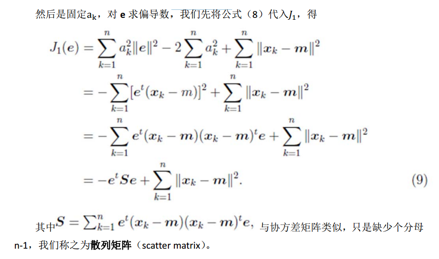
第二步确定方向：

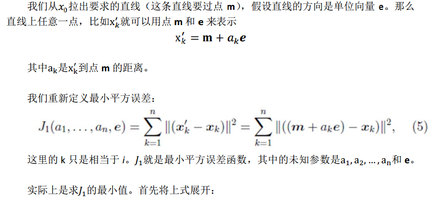
我们首先固定 e，将其看做是常量，||e||=1，然后对$a_k$进行求导，得:

这个结果意思是说，如果知道了 e，那么将$x_k'-m$与$e$做内积，就可以得到$x_k$在$e$上的投影到$m$的距离。

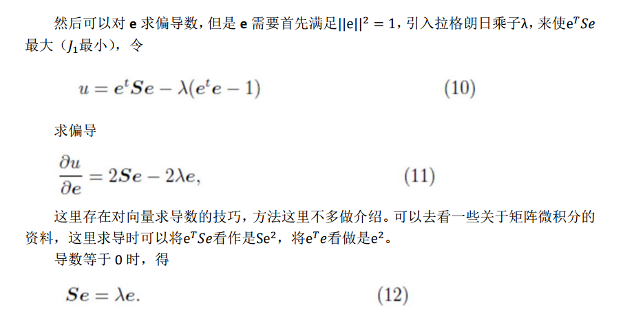
两边除以 n‐1 就变成了，对协方差矩阵求特征值向量了。

从不同的思路出发，最后得到同一个结果，对协方差矩阵求特征向量，求得后特征向量上就成为了新的坐标，如下图：

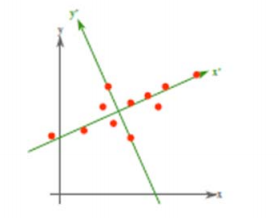
这时候点都聚集在新的坐标轴周围，因为我们使用的最小平方误差的意义就在此。

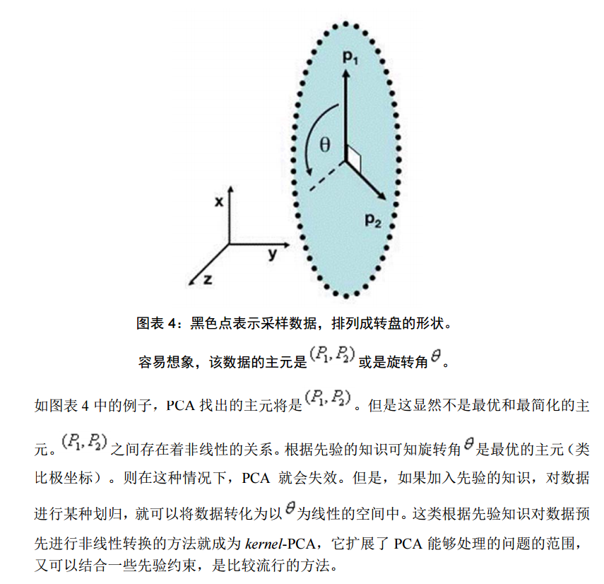
PCA 理论意义

PCA 将 n 个特征降维到 k 个，可以用来进行数据压缩，如果 100 维的向量最后可以用10 维来表示，那么压缩率为 90%。同样图像处理领域的 KL 变换使用 PCA 做图像压缩。但PCA 要保证降维后，还要保证数据的特性损失最小。再看回顾一下 PCA 的效果。经过 PCA处理后，二维数据投影到一维上可以有以下几种情况：

我们认为左图好，一方面是投影后方差最大，一方面是点到直线的距离平方和最小，而且直线过样本点的中心点。为什么右边的投影效果比较差？直觉是因为坐标轴之间相关，以至于去掉一个坐标轴，就会使得坐标点无法被单独一个坐标轴确定。

PCA 得到的 k 个坐标轴实际上是 k 个特征向量，由于协方差矩阵对称，因此 k 个特征向量正交。看下面的计算过程。

我们最后得到的投影结果是AE，E 是 k 个特征向量组成的矩阵，展开如下：

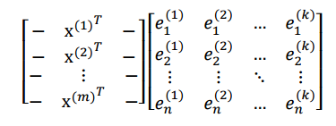
得到的新的样例矩阵就是 m 个样例到 k 个特征向量的投影，也是这 k 个特征向量的线性组合。。e 之间是正交的。从矩阵乘法中可以看出，PCA 所做的变换是将原始样本点（n 维），投影到 k 个正交的坐标系中去，丢弃其他维度的信息。
举个例子，假设宇宙是 n 维的（霍金说是 13 维的），我们得到银河系中每个星星的坐标（相对于银河系中心的 n 维向量），然而我们想用二维坐标去逼近这些样本点，假设算出来的协方差矩阵的特征向量分别是图中的水平和竖直方向，那么我们建议以银河系中心为原点的 x 和 y 坐标轴，所有的星星都投影到 x和 y 上，得到下面的图片。然而我们丢弃了每个星星离我们的远近距离等信息。

总结与讨论

这一部分来自 http://www.cad.zju.edu.cn/home/chenlu/pca.htm

$\bullet$PCA 技术的一大好处是对数据进行降维的处理。我们可以对新求出的“主元”向量的重要性进行排序，根据需要取前面最重要的部分，将后面的维数省去，可以达到降维从而简化模型或是对数据进行压缩的效果。同时最大程度的保持了原有数据的信息。
$\bullet$PCA 技术的一个很大的优点是，它是完全无参数限制的。在 PCA 的计算过程中完全不需要人为的设定参数或是根据任何经验模型对计算进行干预，最后的结果只与数据相关，与用户是独立的。
$\qquad$但是，这一点同时也可以看作是缺点。如果用户对观测对象有一定的先验知识，掌握了数据的一些特征，却无法通过参数化等方法对处理过程进行干预，可能会得不到预期的效果，效率也不高。

其他参考文献

A tutorial on Principal Components Analysis LI Smith – 2002
A Tutorial on Principal Component Analysis J Shlens
http://www.cmlab.csie.ntu.edu.tw/~cyy/learning/tutorials/PCAMissingData.pdf
http://www.cad.zju.edu.cn/home/chenlu/pca.htm

下面的练习来自UFLDL
pca2d

close all

%%================================================================
%% Step 0: Load data
%  We have provided the code to load data from pcaData.txt into x.
%  x is a 2 * 45 matrix, where the kth column x(:,k) corresponds to
%  the kth data point.Here we provide the code to load natural image data into x.
%  You do not need to change the code below.

x = load('pcaData.txt','-ascii');
figure(1);
scatter(x(1, :), x(2, :));
title('Raw data');


%%================================================================
%% Step 1a: Implement PCA to obtain U 
%  Implement PCA to obtain the rotation matrix U, which is the eigenbasis
%  sigma. 

% -------------------- YOUR CODE HERE -------------------- 
u = zeros(size(x, 1)); % You need to compute this
avg = mean(x,2);
x = x - repmat(avg,1,size(x,2));
sigma = x * x' /size(x,2);
[U,S,V] = svd(sigma);
u = U;
% -------------------------------------------------------- 
hold on
plot([0 u(1,1)], [0 u(2,1)]);
plot([0 u(1,2)], [0 u(2,2)]);
scatter(x(1, :), x(2, :));
hold off

%%================================================================
%% Step 1b: Compute xRot, the projection on to the eigenbasis
%  Now, compute xRot by projecting the data on to the basis defined
%  by U. Visualize the points by performing a scatter plot.

% -------------------- YOUR CODE HERE -------------------- 
xRot = zeros(size(x)); % You need to compute this
xRot = u'*x;

% -------------------------------------------------------- 

% Visualise the covariance matrix. You should see a line across the
% diagonal against a blue background.
figure(2);
scatter(xRot(1, :), xRot(2, :));
title('xRot');

%%================================================================
%% Step 2: Reduce the number of dimensions from 2 to 1. 
%  Compute xRot again (this time projecting to 1 dimension).
%  Then, compute xHat by projecting the xRot back onto the original axes 
%  to see the effect of dimension reduction

% -------------------- YOUR CODE HERE -------------------- 
k = 1; % Use k = 1 and project the data onto the first eigenbasis
xHat = zeros(size(x)); % You need to compute this
x_pca = u(:,1)' * x;
xHat = U*[x_pca;zeros(1,size(x,2))];


% -------------------------------------------------------- 
figure(3);
scatter(xHat(1, :), xHat(2, :));
title('xHat');


%%================================================================
%% Step 3: PCA Whitening
%  Complute xPCAWhite and plot the results.

epsilon = 1e-5;
% -------------------- YOUR CODE HERE -------------------- 
xPCAWhite = zeros(size(x)); % You need to compute this

xPCAWhite = diag( 1./sqrt(diag(S)+epsilon) ) * xRot;


% -------------------------------------------------------- 
figure(4);
scatter(xPCAWhite(1, :), xPCAWhite(2, :));
title('xPCAWhite');

%%================================================================
%% Step 3: ZCA Whitening
%  Complute xZCAWhite and plot the results.

% -------------------- YOUR CODE HERE -------------------- 
xZCAWhite = zeros(size(x)); % You need to compute this
xZCAWhite = U * xPCAWhite;

% -------------------------------------------------------- 
figure(5);
scatter(xZCAWhite(1, :), xZCAWhite(2, :));
title('xZCAWhite');

%% Congratulations! When you have reached this point, you are done!
%  You can now move onto the next PCA exercise. :)

pca_gen

%%================================================================
%% Step 0a: Load data
%  Here we provide the code to load natural image data into x.
%  x will be a 144 * 10000 matrix, where the kth column x(:, k) corresponds to
%  the raw image data from the kth 12x12 image patch sampled.
%  You do not need to change the code below.

x = sampleIMAGESRAW();
figure('name','Raw images');
randsel = randi(size(x,2),200,1); % A random selection of samples for visualization
display_network(x(:,randsel));%这里只显示了部分子样本

%%================================================================
%% Step 0b: Zero-mean the data (by row)
%  You can make use of the mean and repmat/bsxfun functions.

% -------------------- YOUR CODE HERE -------------------- 
[n,m] = size(x)  %n是属性，m是样本数
avg_features = mean(x,2) %求得每一维特征的均值  2代表按行求均值
x = x - repmat(avg_features, 1, size(x,2));
display_network(x(:,randsel));%做0均值前后的对比

%%================================================================
%% Step 1a: Implement PCA to obtain xRot
%  Implement PCA to obtain xRot, the matrix in which the data is expressed
%  with respect to the eigenbasis of sigma, which is the matrix U.


% -------------------- YOUR CODE HERE -------------------- 
xRot = zeros(size(x)); % You need to compute this
sigma = x*x'/size(x,2);
[U,S,V] = svd(sigma)%计算特征向量 U特征向量构成的矩阵，特征向量数与属性数相同，第一个特征向量与某个样本相乘解a1*x1得xRot中样本x1的第一个属性，S特征值
xRot = U' * x; 
%%================================================================
%% Step 1b: Check your implementation of PCA
%  The covariance matrix for the data expressed with respect to the basis U
%  should be a diagonal matrix with non-zero entries only along the main
%  diagonal. We will verify this here.
%  Write code to compute the covariance matrix, covar. 
%  When visualised as an image, you should see a straight line across the
%  diagonal (non-zero entries) against a blue background (zero entries).

% -------------------- YOUR CODE HERE -------------------- 
covar = zeros(size(x, 1)); % You need to compute this
covar = xRot*xRot';%协方差是属性间的协方差，不是每个样本的协方差
% Visualise the covariance matrix. You should see a line across the
% diagonal against a blue background.
figure('name','Visualisation of covariance matrix');
imagesc(covar);

%%================================================================
%% Step 2: Find k, the number of components to retain
%  Write code to determine k, the number of components to retain in order
%  to retain at least 99% of the variance.

% -------------------- YOUR CODE HERE -------------------- 
k = 0; % Set k accordingly
var_sum = sum(diag(covar));%covar主对角线上就是特征值
curr_var_sum = 0;
for i = 1:length(covar)
   curr_var_sum = curr_var_sum + covar(i,i); 
   if curr_var_sum / var_sum >= 0.99
       k=i;
       break;
   end
end

%%================================================================
%% Step 3: Implement PCA with dimension reduction
%  Now that you have found k, you can reduce the dimension of the data by
%  discarding the remaining dimensions. In this way, you can represent the
%  data in k dimensions instead of the original 144, which will save you
%  computational time when running learning algorithms on the reduced
%  representation.
% 
%  Following the dimension reduction, invert the PCA transformation to produce 
%  the matrix xHat, the dimension-reduced data with respect to the original basis.
%  Visualise the data and compare it to the raw data. You will observe that
%  there is little loss due to throwing away the principal components that
%  correspond to dimensions with low variation.

% -------------------- YOUR CODE HERE -------------------- 
xHat = zeros(size(x));  % You need to compute this
xTitle = U(:,1:k)' * x; %这个是pca降维后的结果
xHat = U*[xTitle;zeros(n-k,m)];%由pca后的数据恢复原图

% Visualise the data, and compare it to the raw data
% You should observe that the raw and processed data are of comparable quality.
% For comparison, you may wish to generate a PCA reduced image which
% retains only 90% of the variance.

figure('name',['PCA processed images ',sprintf('(%d / %d dimensions)', k, size(x, 1)),'']);
display_network(xHat(:,randsel));
figure('name','Raw images');
display_network(x(:,randsel));

%%================================================================
%% Step 4a: Implement PCA with whitening and regularisation
%  Implement PCA with whitening and regularisation to produce the matrix
%  xPCAWhite. 

epsilon = 0.1;
xPCAWhite = zeros(size(x));

% -------------------- YOUR CODE HERE -------------------- 
xPCAWhite = diag(1./sqrt(diag(S) + epsilon)) * xRot;
%%================================================================
%% Step 4b: Check your implementation of PCA whitening 
%  Check your implementation of PCA whitening with and without regularisation. 
%  PCA whitening without regularisation results a covariance matrix 
%  that is equal to the identity matrix. PCA whitening with regularisation
%  results in a covariance matrix with diagonal entries starting close to 
%  1 and gradually becoming smaller. We will verify these properties here.
%  Write code to compute the covariance matrix, covar. 
%
%  Without regularisation (set epsilon to 0 or close to 0), 
%  when visualised as an image, you should see a red line across the
%  diagonal (one entries) against a blue background (zero entries).
%  With regularisation, you should see a red line that slowly turns
%  blue across the diagonal, corresponding to the one entries slowly
%  becoming smaller.

% -------------------- YOUR CODE HERE -------------------- 
covar = xPCAWhite * xPCAWhite';
% Visualise the covariance matrix. You should see a red line across the
% diagonal against a blue background.
figure('name','Visualisation of covariance matrix');
imagesc(covar);

%%================================================================
%% Step 5: Implement ZCA whitening
%  Now implement ZCA whitening to produce the matrix xZCAWhite. 
%  Visualise the data and compare it to the raw data. You should observe
%  that whitening results in, among other things, enhanced edges.

xZCAWhite = zeros(size(x));%ZCA白化一般都作用于所有维度，数据不降维
xZCAWhite = U * xPCAWhite; %ZCA其实就是做了PCA白化后再复原原图---增强边缘
% -------------------- YOUR CODE HERE -------------------- 

% Visualise the data, and compare it to the raw data.
% You should observe that the whitened images have enhanced edges.
figure('name','ZCA whitened images');
display_network(xZCAWhite(:,randsel));
figure('name','Raw images');
display_network(x(:,randsel));

使用pca的基本步骤是
输入x—对x做零均值—计算x的协方差矩阵—计算特征值特征向量—-白化（可选，它可消除样本间的相关性）—-选取前k个特征向量