python学习--模型过拟合查看learning curve

参考：http://blog.csdn.net/han_xiaoyang/article/details/49797143

学习曲线是什么
学习曲线是不同训练集大小，模型在训练集和验证集上的得分变化曲线。也就是以样本数为横坐标，训练和交叉验证集上的得分（如准确率）为纵坐标。learning curve可以帮助我们判断模型现在所处的状态：过拟合（overfiting / high variance） or 欠拟合（underfitting / high bias）
模型欠拟合、过拟合、偏差和方差平衡 时对应的学习曲线如下图所示：

怎么看学习曲线
左上角的图中训练集和验证集上的曲线能够收敛。在训练集合验证集上准确率相差不大，却都很差。这说明模拟对已知数据和未知都不能进行准确的预测，属于高偏差。这种情况模型很可能是欠拟合。可以针对欠拟合采取对应的措施。

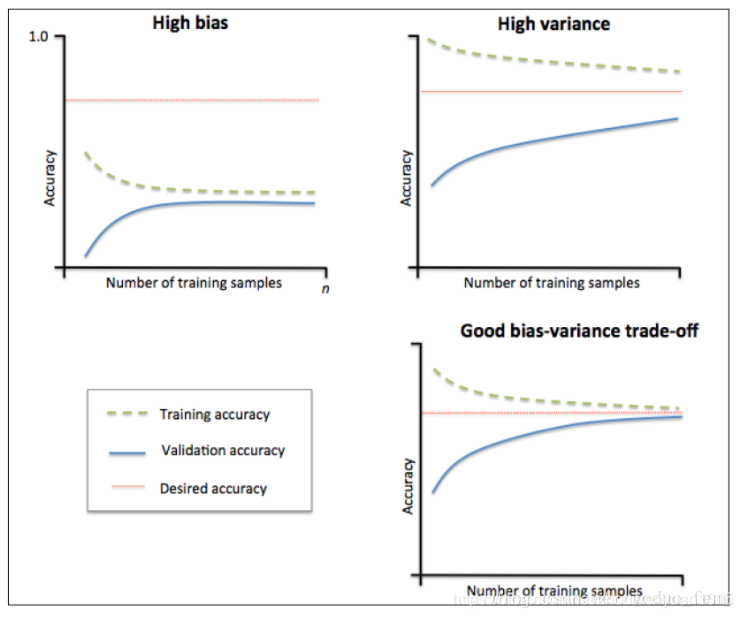
右上角的图中模型在训练集上和验证集上的准确率差距很大。说明模型能够很好的拟合已知数据，但是泛化能力很差，属于高方差。模拟很可能过拟合，要采取过拟合对应的措施

以上 原文链接：https://blog.csdn.net/geduo_feng/article/details/79547554

功能说明：

查看模型是否过拟合：
一般过拟合：随着样本量增加，准确率在训练集上得分比较高，交叉验证集上得分较小，中间gab较大。

参数说明：

rain_sizes, train_scores, test_scores = learning_curve(
输入：
    (estimator : 你用的分类器。
    title : 表格的标题。
    X : 输入的feature，numpy类型
    y : 输入的target vector
    ylim : tuple格式的(ymin, ymax), 设定图像中纵坐标的最低点和最高点
    cv : 做cross-validation的时候，数据分成的份数，其中一份作为cv集，其余n-1份作为training(默认为3份)
    n_jobs : 并行的的任务数(默认1))
输出：(train_sizes_abs :训练样本数
      train_scores:训练集上准确率
      test_scores:交叉验证集上的准确率)    

python示例:

from sklearn.naive_bayes import GaussianNB
import numpy as np
from sklearn.learning_curve import learning_curve #c查看是否过拟合

def plot_learning_curve(estimator, title, X, y, ylim=None, cv=None, n_jobs=1, train_sizes=np.linspace(.05, 1., 20), verbose=0, plot=True):
    """
    画出data在某模型上的learning curve.
    参数解释
    ----------
    estimator : 你用的分类器。
    title : 表格的标题。
    X : 输入的feature，numpy类型
    y : 输入的target vector
    ylim : tuple格式的(ymin, ymax), 设定图像中纵坐标的最低点和最高点
    cv : 做cross-validation的时候，数据分成的份数，其中一份作为cv集，其余n-1份作为training(默认为3份)
    n_jobs : 并行的的任务数(默认1)
    """
    train_sizes, train_scores, test_scores = learning_curve(
        estimator, X, y, cv=cv, n_jobs=n_jobs, train_sizes=train_sizes, verbose=verbose)

    train_scores_mean = np.mean(train_scores, axis=1)
    train_scores_std = np.std(train_scores, axis=1)
    test_scores_mean = np.mean(test_scores, axis=1)
    test_scores_std = np.std(test_scores, axis=1)

    if plot:
        plt.figure()
        plt.title(title)
        if ylim is not None:
            plt.ylim(*ylim)
        plt.xlabel(u"train_sample")
        plt.ylabel(u"score")
        plt.gca().invert_yaxis()
        plt.grid()

        plt.fill_between(train_sizes, train_scores_mean - train_scores_std, train_scores_mean + train_scores_std, 
                         alpha=0.1, color="b")
        plt.fill_between(train_sizes, test_scores_mean - test_scores_std, test_scores_mean + test_scores_std, 
                         alpha=0.1, color="r")
        plt.plot(train_sizes, train_scores_mean, 'o-', color="b", label=u"train_score")
        plt.plot(train_sizes, test_scores_mean, 'o-', color="r", label=u"cross_validation_score")

        plt.legend(loc="best")

        plt.draw()
        plt.show()
        plt.gca().invert_yaxis()
        plt.savefig("learn_curve.jpg") 

    midpoint = ((train_scores_mean[-1] + train_scores_std[-1]) + (test_scores_mean[-1] - test_scores_std[-1])) / 2
    diff = (train_scores_mean[-1] + train_scores_std[-1]) - (test_scores_mean[-1] - test_scores_std[-1])
    return midpoint, diff
if __name__=='__main__':
X=np.array([[ 1.        , -0.12493874,  0.04575749],
       [ 0.        , -0.30103   ,  0.03140846],
       [ 1.        , -0.17609126,  0.11394335],
       [ 1.        , -0.30103   , -0.06694679],
       [ 1.        , -0.30103   , -0.12104369],
       [ 1.        , -0.23408321,  0.11270428],
       [ 1.        ,  0.19188553,  0.22577904],
       [ 1.        , -0.23736092, -0.42100531],
       [ 0.        ,  0.21085337,  0.13966199],
       [ 1.        , -0.06214791,  0.07716595],
       [ 1.        ,  0.14612804, -0.01223446],
       [ 1.        ,  0.1383027 ,  0.1217336 ],
       [ 1.        , -0.30103   , -0.18073616],
       [ 0.        ,  0.02996322, -0.09108047],
       [ 0.        ,  0.05435766,  0.1638568 ],
       [ 1.        , -0.11394335,  0.        ],
       [ 1.        ,  0.06694679,  0.30998484],
       [ 0.        ,  0.64345268,  0.02802872],
       [ 1.        ,  0.        , -0.01639042],
       [ 0.        ,  0.11394335, -0.0234811 ],
       [ 0.        ,  0.        ,  0.18799048],
       [ 1.        ,  0.        ,  0.10914447],
       [ 1.        , -0.04139269,  0.        ],
       [ 0.        ,  0.18905624,  0.17026172],
       [ 1.        , -0.14132915,  0.15209098],
       [ 0.        ,  0.30103   ,  0.27036118],
       [ 1.        ,  0.22184875,  0.05435766],
       [ 0.        ,  0.34242268,  0.09455611],
       [ 1.        , -0.20411998, -0.1173856 ],
       [ 0.        ,  0.11394335,  0.01189922],
       [ 1.        , -0.22184875, -0.01378828],
       [ 1.        ,  0.13262557,  0.14390658],
       [ 0.        ,  0.14612804,  0.13353891]])
       
y=np.array([1, 0, 1, 1, 1, 1, 0, 1, 0, 0, 1, 0, 1, 1, 1, 0, 0, 0, 1, 0, 1, 1, 1,
       0, 1, 0, 0, 0, 1, 0, 1, 0, 0])

Gmodel=GaussianNB()
train_sizes, train_scores, test_scores=learning_curve(Gmodel,X,y,train_sizes=[3,6,10],cv=3)
plot_learning_curve(Gmodel, u"learning curve", X, y)

数据结果

注：测试样本量较少，在样本量为10处存在一些过拟合