【Paddle】超越 attention：RWKV-7 架构的 Paddle 实现

要直接运行本项目，可以前往飞桨星河平台一键运行。

RWKV 简介

• RWKV（读作 RWaKuV）是一种具有 GPT 级大型语言模型（LLM）性能的 RNN，也可以像 GPT Transformer 一样直接训练（可并行化）。

• RWKV 结合了 RNN 和 Transformer 的最佳特性：出色的性能、恒定的显存占用、恒定的推理生成速度、“无限” ctxlen 和免费的句嵌入，而且 100% 不含自注意力机制。

• RWKV 项目最初由彭博（Bo Peng ，BlinkDL）提出，随着项目被外界关注，RWKV 项目逐渐发展成一个开源社区。

• 最新 RWKV 论文可见：RWKV-7 “Goose” with Expressive Dynamic State Evolution

项目说明

本项目使用纯 Paddle 实现了国产纯 RNN 大模型架构 RWKV-7，并和 Paddle 封装的 Transformer 进行了对比，同时为了增强实验的可靠性，将 LSTM 也加入了对比，具体对比维度如下表：

对比维度	RWKV-7	Transformer	LSTM
参数量 (Parameters)	~3.1 万 (30,732)	~3.0 万 (30,380)	~87.7 万 (877,452)
层数 (Layers)	2 层	2 层	7 层
隐藏层维度 (Dim)	32	32	128
核心机制	RNN ($O(1)$)	Self-Attention ($O(T)$)	Gated RNN (串行)
位置编码	不需要 (自带 Time Decay)	需要 (Learned Embedding)	不需要 (隐式时序)
训练并行性	高 (类 Transformer 并行模式)	高 (可并行计算所有 token)	低 (必须串行计算 t0->t1…)
推理复杂度	$O(1)$ (固定 State 显存占用)	$O(T)$ (KV Cache 随长度增长)	$O(1)$ (固定 Hidden State)
训练数据规模	256 万条 / 3.28 亿 Token	256 万条 / 3.28 亿 Token	256 万条 / 3.28 亿 Token
学习率调节方式	余弦退火	余弦退火	固定学习率
实验公平性	公平 (同规模对比)	公平 (同规模对比)	不公平 (参数量大 30 倍)

（在项目最后搭建了 MLP 进行对比，但由于 MLP 无法学习时序类的规则任务，在本项目测试任务中效果极差，因此未加入对比）

数据和评测任务

1. 核心任务：教模型“倒背数字”。
2. 数据示例：12345 (看到逗号) -> 54321 (倒着背出来) -> # (结束)。
3. 词表很小：模型只认识 12 个符号（0到9，逗号，井号）。
4. 数据量大：模型一共练习了 256 万次，看了 3.2 亿 个字符。
5. 实时生成：数据是代码现场随机造的，没有存成文件。
6. 难度：数字最长有 60 位，模型必须拥有“长距离记忆”才能背对。

指标计算方法

• AC 率（正确率）：逐位计算，正确 1 位则记录 1 位的 AC 率，而非要求整个序列正确（整个序列都对才算对的话，要爆 0 了）
• loss：经典的交叉熵损失

为什么这里的 RWKV-7 会慢很多？

• 因为我不会写 Paddle 的 CUDA 算子，所以此处没有加速实现，相较于使用了 CUDA 算子的 torch 版 RWKV-7，此处的速度慢约 95%（RWKV-LM 仓库的 rwkv7_train_simplified.py 是本项目测试内容的官方实现，约 3 分钟可以完成本项目中的 RWKV 模型训练)；
• LSTM 和 Transformer 使用 Paddle 官方封装好的模型，本身包含 CUDA 算子加速，因此是加速后的速度；

项目复现说明

• 直接运行本 notebook 即可，注意使用有 CUDA 的环境，虽然本项目不含自定义的 CUDA 算子，但代码仍使用了封装好的接口调用 CUDA，Transformer 和 LSTM 直接使用了 Paddle 封装的方法，在飞桨的其他平台应该也有加速，但未做特殊指定，建议使用 Nvidia 显卡（飞桨平台上的 V100 或 A100 ）；

• 运行全部内容需要约 1 小时，每天飞桨免费的算力完全足够复现本项目；

实测结果

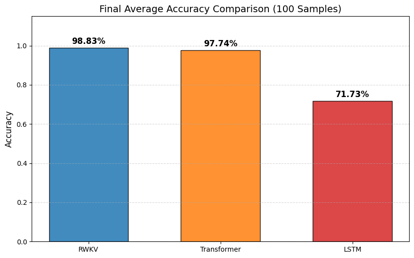
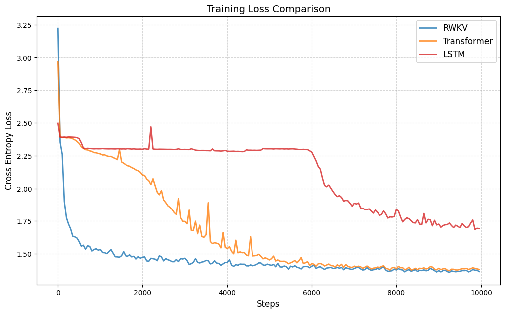
下面是三个模型的 loss 下降对比和测试集 AC 率对比，LSTM 可以学到一定程度的“倒背数字”，RWKV-7 和 Transformer 可以基本学会“倒背数字”，且 RWKV-7 的 loss 下降更稳定的同时且更快，并且 RWKV-7 的 AC 率更高。

测试代码

RWKV-7

import random
import os
import math
import time
import datetime
import csv
import numpy as np
from types import SimpleNamespace
import paddle
from paddle import nn
import paddle.nn.functional as F

# === 绘图与可视化依赖 ===
import matplotlib
matplotlib.use('Agg') 
import matplotlib.pyplot as plt
from IPython.display import Image, display

# === 设备配置 ===
if paddle.device.is_compiled_with_cuda():
    paddle.set_device('gpu')
else:
    paddle.set_device('cpu')

def set_seed_all(seed):
    """固定随机种子，确保训练过程可复现"""
    paddle.seed(seed)
    random.seed(seed)
    np.random.seed(seed)

set_seed_all(42)

# === 全局超参数定义 ===
V = 12             # 词表大小 (Vocab Size): 0-9数字 + ',' + '#'
C = 32             # 嵌入维度 (Embedding Dimension): 通道数/隐藏层大小
B = 256            # 批次大小 (Batch Size)
T = 129            # 序列长度 (Context Length): 输入序列的最大长度
steps = 10000      # 训练迭代步数
lr0 = 4e-3         # 初始学习率
lr1 = 1e-6         # 最小学习率 (Cosine Decay 终点)
DIGIT_MAX = 60     # 数据生成任务中，数字的最大位数
HEAD_SIZE = 16     # 注意力头维度 (Head Dimension)

# === 日志与输出路径 ===
LOG_DIR = "logs"
os.makedirs(LOG_DIR, exist_ok=True)

# === 核心算子: RWKV-7 State Mixing (RNN 核心递归单元) ===
class RWKV7_Core(nn.Layer):
    """
    RWKV v7 的核心循环单元。
    实现类似于线性注意力的递归更新逻辑，但在 RWKV7 中引入了更复杂的 state 更新机制。
    """
    def __init__(self):
        super().__init__()

    def forward(self, w, q, k, v, a, b):
        """
        参数说明 (B: Batch, T: Time, H: Head, C: Head_Dim):
        w: [B, T, H, C] - 衰减因子 (Decay), 控制历史信息的保留程度
        q: [B, T, H, C] - 查询向量 (Query)
        k: [B, T, H, C] - 键向量 (Key)
        v: [B, T, H, C] - 值向量 (Value)
        a: [B, T, H, C] - 更新因子 A (用于 v7 特定状态更新)
        b: [B, T, H, C] - 更新因子 B (用于 v7 特定状态更新)
        """
        B, T, H, C = w.shape
        
        # 将 w 转换为对数空间的衰减率，保证数值稳定性 (-exp(w) 确保为负数，再取 exp 得到 (0, 1) 区间的衰减)
        w = paddle.exp(-paddle.exp(w))

        # 调整维度以适应时间步循环 [T, B, H, C]
        w = w.transpose([1, 0, 2, 3]); q = q.transpose([1, 0, 2, 3])
        k = k.transpose([1, 0, 2, 3]); v = v.transpose([1, 0, 2, 3])
        a = a.transpose([1, 0, 2, 3]); b = b.transpose([1, 0, 2, 3])

        # 初始化隐藏状态 State: [B, H, C, C] (类似于 KV Cache，但在 RWKV 中是固定大小的矩阵)
        state = paddle.zeros([B, H, C, C], dtype=w.dtype)
        y_list = []

        # === 时间步递归计算 (核心串行部分) ===
        for t in range(T):
            wt = w[t]; qt = q[t]; kt = k[t]; vt = v[t]; at = a[t]; bt = b[t]

            # 1. 计算状态注意力分数 sa
            # sa = (State * at).sum -> 将当前状态与因子 a 交互，聚合信息
            sa = (state * at.unsqueeze(2)).sum(axis=-1, keepdim=True)

            # 2. 状态更新 (RWKV7 特有的更新规则)
            # term1: 历史状态衰减 (State * w)
            term1 = state * wt.unsqueeze(2)
            # term2: 状态交互项 (sa * b)
            term2 = sa * bt.unsqueeze(2)
            # term3: 新信息注入 (v * k)，类似于标准的 KV 写入
            term3 = vt.unsqueeze(3) * kt.unsqueeze(2)
            
            state = term1 + term2 + term3  # 更新状态矩阵

            # 3. 计算当前时刻输出
            # output = (State * q).sum -> 从状态中根据 Query 读取信息
            yt = (state * qt.unsqueeze(2)).sum(axis=-1)
            y_list.append(yt)
        
        y = paddle.stack(y_list, axis=0) # [T, B, H, C]
        return y.transpose([1, 0, 2, 3]) # [B, T, H, C]

global_rwkv_core = RWKV7_Core()

def RUN_PADDLE_RWKV7g(q, w, k, v, a, b):
    """
    RWKV7 Core 的包装函数，处理 Head 和 Channel 的维度重塑。
    将总通道数 HC 拆分为 H 个头，每个头大小为 C=16 (在 RWKV7 中通常固定为 16 或 64)
    """
    B, T, HC = q.shape
    H = HC // 16; C = 16 
    # 重塑为 [B, T, H, C] 以输入到核心算子
    q = q.reshape([B, T, H, C]); w = w.reshape([B, T, H, C])
    k = k.reshape([B, T, H, C]); v = v.reshape([B, T, H, C])
    a = a.reshape([B, T, H, C]); b = b.reshape([B, T, H, C])
    
    y = global_rwkv_core(w, q, k, v, a, b)
    
    return y.reshape([B, T, HC]) # 还原为 [B, T, HC]

# === RWKV Time Mixing 层 (混合时间维度的信息) ===
class RWKV_Tmix_x070(nn.Layer):
    def __init__(self, args, layer_id):
        super().__init__()
        self.args = args; self.layer_id = layer_id
        self.head_size = args.head_size
        self.n_head = args.dim_att // self.head_size
        H = self.n_head; N = self.head_size; C = args.n_embd

        # 计算层深比例，用于初始化参数的缩放
        ratio_0_to_1 = layer_id / (args.n_layer - 1)
        ratio_1_to_almost0 = 1.0 - (layer_id / args.n_layer)

        # === 初始化 Time-Mix 差值参数 (Learned Interpolation) ===
        # ddd: 用于参数初始化的辅助张量
        ddd_np = np.ones((1, 1, C), dtype='float32')
        for i in range(C): ddd_np[0, 0, i] = i / C
        ddd = paddle.to_tensor(ddd_np)

        # x_r, x_w, x_k... : 对应 r, w, k, v, a, g 各个门的 token 混合系数
        # 用于混合当前时刻 t 和上一时刻 t-1 的输入
        self.x_r = self.create_parameter(shape=[1, 1, C], default_initializer=nn.initializer.Assign(1.0 - paddle.pow(ddd, 0.2 * ratio_1_to_almost0)))
        self.x_w = self.create_parameter(shape=[1, 1, C], default_initializer=nn.initializer.Assign(1.0 - paddle.pow(ddd, 0.9 * ratio_1_to_almost0)))
        self.x_k = self.create_parameter(shape=[1, 1, C], default_initializer=nn.initializer.Assign(1.0 - paddle.pow(ddd, 0.7 * ratio_1_to_almost0)))
        self.x_v = self.create_parameter(shape=[1, 1, C], default_initializer=nn.initializer.Assign(1.0 - paddle.pow(ddd, 0.7 * ratio_1_to_almost0)))
        self.x_a = self.create_parameter(shape=[1, 1, C], default_initializer=nn.initializer.Assign(1.0 - paddle.pow(ddd, 0.9 * ratio_1_to_almost0)))
        self.x_g = self.create_parameter(shape=[1, 1, C], default_initializer=nn.initializer.Assign(1.0 - paddle.pow(ddd, 0.2 * ratio_1_to_almost0)))

        # 辅助函数：正交初始化
        def ortho_init(shape, scale):
            flat_shape = (shape[0], np.prod(shape[1:])) if len(shape) > 2 else shape
            rows, cols = flat_shape
            a = np.random.normal(0.0, 1.0, flat_shape).astype('float32')
            if rows < cols: a = a.T
            q, r = np.linalg.qr(a)
            d = np.diag(r, 0); q *= np.sign(d)
            if rows < cols: q = q.T
            q = q[:rows, :cols] if rows > cols else q
            q = q.reshape(shape)
            return paddle.to_tensor(q * scale)

        # === 初始化 Low-Rank Adapter 参数 (用于生成 w, a, v, g 的动态变化) ===
        # 这里使用了特定于 RWKV 的各种初始化策略 (Zigzag, Linear 等) 以优化训练收敛
        www = np.zeros(C, dtype='float32'); zigzag = np.zeros(C, dtype='float32'); linear = np.zeros(C, dtype='float32')
        for n in range(C):
            linear[n] = n / (C-1) - 0.5
            z_val = ((n % N) - ((N-1) / 2)) / ((N-1) / 2)
            zigzag[n] = z_val * abs(z_val)
            www[n] = -6 + 6 * (n / (C - 1)) ** (1 + 1 * ratio_0_to_1 ** 0.3)
        www = paddle.to_tensor(www); zigzag = paddle.to_tensor(zigzag); linear = paddle.to_tensor(linear)

        # 定义生成各个门的 LoRA (Low-Rank) 权重
        self.w1 = self.create_parameter(shape=[C, 8], default_initializer=nn.initializer.Constant(0.0))
        self.w2 = self.create_parameter(shape=[8, C], default_initializer=nn.initializer.Assign(ortho_init((8, C), 0.1)))
        self.w0 = self.create_parameter(shape=[1, 1, C], default_initializer=nn.initializer.Assign(www.reshape([1,1,C]) + 0.5 + zigzag*2.5))
        
        self.a1 = self.create_parameter(shape=[C, 8], default_initializer=nn.initializer.Constant(0.0))
        self.a2 = self.create_parameter(shape=[8, C], default_initializer=nn.initializer.Assign(ortho_init((8, C), 0.1)))
        self.a0 = self.create_parameter(shape=[1, 1, C], default_initializer=nn.initializer.Assign(paddle.zeros([1,1,C])-0.19 + zigzag*0.3 + linear*0.4))
        
        self.v1 = self.create_parameter(shape=[C, 8], default_initializer=nn.initializer.Constant(0.0))
        self.v2 = self.create_parameter(shape=[8, C], default_initializer=nn.initializer.Assign(ortho_init((8, C), 0.1)))
        self.v0 = self.create_parameter(shape=[1, 1, C], default_initializer=nn.initializer.Assign(paddle.zeros([1,1,C])+0.73 - linear*0.4))
        
        self.g1 = self.create_parameter(shape=[C, 8], default_initializer=nn.initializer.Constant(0.0))
        self.g2 = self.create_parameter(shape=[8, C], default_initializer=nn.initializer.Assign(ortho_init((8, C), 0.1)))
        
        self.k_k = self.create_parameter(shape=[1, 1, C], default_initializer=nn.initializer.Assign(paddle.zeros([1,1,C])+0.71 - linear*0.1))
        self.k_a = self.create_parameter(shape=[1, 1, C], default_initializer=nn.initializer.Assign(paddle.zeros([1,1,C])+1.02))
        self.r_k = self.create_parameter(shape=[H, N], default_initializer=nn.initializer.Constant(-0.04))

        # 主要的线性投影层
        self.receptance = nn.Linear(C, C, bias_attr=False) # 接收门 (R)
        self.key = nn.Linear(C, C, bias_attr=False)        # 键 (K)
        self.value = nn.Linear(C, C, bias_attr=False)      # 值 (V)
        self.output = nn.Linear(C, C, bias_attr=False)     # 输出投影 (O)
        self.ln_x = nn.GroupNorm(H, C, epsilon=64e-5)      # GroupNorm 用于归一化状态输出

        # 线性层初始化
        nn.initializer.Uniform(-0.5/(C**0.5), 0.5/(C**0.5))(self.receptance.weight)
        nn.initializer.Uniform(-0.05/(C**0.5), 0.05/(C**0.5))(self.key.weight)
        nn.initializer.Uniform(-0.5/(C**0.5), 0.5/(C**0.5))(self.value.weight)
        nn.initializer.Constant(0.0)(self.output.weight)

    def forward(self, x, v_first=None):
        B, T, C = x.shape; H = self.n_head
        
        # === 1. Time Shift (Token Shift) ===
        # 计算 x 的差分 xx = x[t] - x[t-1]
        xx = paddle.concat([paddle.zeros([B, 1, C], dtype=x.dtype), x[:, :-1, :]], axis=1) - x
        
        # 通过线性插值生成各个门的输入向量
        xr = x + xx * self.x_r; xw = x + xx * self.x_w; xk = x + xx * self.x_k
        xv = x + xx * self.x_v; xa = x + xx * self.x_a; xg = x + xx * self.x_g

        # === 2. 计算各个 Gate 和向量 ===
        r = self.receptance(xr) # Receptance Gate
        
        # Decay (w) 计算: 复杂的非线性变换，确保 w 动态适应上下文
        w = -F.softplus(-(self.w0 + paddle.tanh(xw @ self.w1) @ self.w2), beta=1, threshold=20) - 0.5
        
        k = self.key(xk); v = self.value(xv)
        
        # 这里的逻辑用于处理第一层与后续层的 Skip Connection 或状态传递
        if self.layer_id == 0: v_first = v
        else: v = v + (v_first - v) * F.sigmoid(self.v0 + (xv @ self.v1) @ self.v2)
        
        # 计算 a (in-context 因子) 和 g (gating 因子)
        a = F.sigmoid(self.a0 + (xa @ self.a1) @ self.a2)
        g = F.sigmoid(xg @ self.g1) @ self.g2

        # 归一化和调整 Key
        kk = k * self.k_k
        kk = F.normalize(kk.reshape([B, T, H, -1]), axis=-1, p=2.0, epsilon=1e-12).reshape([B, T, C])
        k = k * (1 + (a-1) * self.k_a)

        # === 3. 调用核心算子 (Bi-Linear Attention) ===
        # 输入: r, w, k, v, -kk (负Key), kk*a (加权Key)
        x = RUN_PADDLE_RWKV7g(r, w, k, v, -kk, kk*a)

        # === 4. 输出处理 ===
        x = self.ln_x(x.reshape([B * T, C])).reshape([B, T, C]) # GroupNorm
        # 加上额外的残差项 (类似于 Attention 中的 Bonus term)
        x = x + ((r.reshape([B,T,H,-1]) * k.reshape([B,T,H,-1]) * self.r_k).sum(axis=-1, keepdim=True) * v.reshape([B,T,H,-1])).reshape([B,T,C])
        
        # 门控输出
        x = self.output(x * g)
        return x, v_first

# === 数据生成逻辑 ===
TOK = {**{str(i):i for i in range(10)}, ',':10, '#':11}
def _digits(n): return [TOK[c] for c in str(n)]

def batch(B, T):
    """
    生成训练批次数据。
    任务：给定一个数字序列，生成其逗号分隔后的逆序。
    格式：[数字] + ',' + [逆序数字] + '#'
    """
    s = []
    for _ in range(B):
        a = []
        while len(a) < T:
            k = random.randint(1, DIGIT_MAX) # 随机位数
            lo = 0 if k==1 else 10**(k-1)
            n = random.randint(lo, 10**k-1); nn_list = _digits(n)
            # 拼接: 原数字 + 逗号 + 逆序数字 + 结束符
            a += nn_list + [TOK[',']] + nn_list[::-1] + [TOK['#']]
        s.append(a[:T])
    return paddle.to_tensor(s, dtype='int64')

# === FFN (Channel Mixing) 层 ===
class FFN(nn.Layer):
    """
    RWKV 的前馈网络层 (Channel Mixing)。
    结构: Input -> TimeShift -> Linear(Expansion) -> ReLU^2 -> Linear(Projection)
    """
    def __init__(self, C):
        super().__init__()
        self.x_k = self.create_parameter(shape=[1, 1, C], default_initializer=nn.initializer.Constant(0.0))
        self.key = nn.Linear(C, C * 4, bias_attr=False)   # 升维 4x
        self.value = nn.Linear(C * 4, C, bias_attr=False) # 降维回 C
        nn.initializer.Constant(0.0)(self.value.weight)
        nn.initializer.Normal(std=0.1)(self.key.weight) 
        
    def forward(self, x):
        B, T, C = x.shape
        # Time Shift: 混合当前 token 和前一个 token
        xx = paddle.concat([paddle.zeros([B, 1, C], dtype=x.dtype), x[:, :-1, :]], axis=1) - x
        x = x + xx * self.x_k
        
        # 激活函数: ReLU 的平方 (Squared ReLU)
        x = paddle.pow(F.relu(self.key(x)), 2)
        return self.value(x)

# === 整体模型结构 ===
class MODEL(nn.Layer):
    def __init__(self):
        super().__init__()
        # 构建参数命名空间
        args = SimpleNamespace(n_head=C // HEAD_SIZE, head_size=HEAD_SIZE, n_embd=C, dim_att=C, n_layer=2)
        
        self.e = nn.Embedding(V, C)             # 词嵌入
        self.ln1a = nn.LayerNorm(C); self.ln1b = nn.LayerNorm(C) # Pre-LN
        self.rwkv1 = RWKV_Tmix_x070(args, 0); self.ffn1 = FFN(C) # Layer 1
        
        self.ln2a = nn.LayerNorm(C); self.ln2b = nn.LayerNorm(C)
        self.rwkv2 = RWKV_Tmix_x070(args, 1); self.ffn2 = FFN(C) # Layer 2
        
        self.lno = nn.LayerNorm(C)              # Final LN
        self.o = nn.Linear(C, V, bias_attr=True)# 输出层 (Logits)

    def forward(self, x):
        x = self.e(x)
        
        # Block 1: Attention (TimeMix) + FFN (ChannelMix)
        xx, v_first = self.rwkv1(self.ln1a(x), None)
        x = x + xx
        x = x + self.ffn1(self.ln1b(x))
        
        # Block 2
        xx, v_first = self.rwkv2(self.ln2a(x), v_first)
        x = x + xx
        x = x + self.ffn2(self.ln2b(x))
        
        x = self.o(self.lno(x))
        return x

# === 模型初始化与优化器配置 ===
model = MODEL()

# 分组参数以应用不同的权重衰减 (Weight Decay)
decay = []; no_decay = []
for n, p in model.named_parameters():
    if p.stop_gradient: continue
    # 对权重参数应用衰减，对 Bias 和 LayerNorm 参数不应用衰减
    if ('.weight' in n or 'emb' in n) and ('ln' not in n): decay.append(p)
    else: no_decay.append(p)

# 学习率调度: 余弦退火
scheduler = paddle.optimizer.lr.CosineAnnealingDecay(learning_rate=lr0, T_max=steps, eta_min=lr1)
# 优化器: AdamW
opt = paddle.optimizer.AdamW(parameters=[{'params': decay, 'weight_decay': 0.1}, {'params': no_decay, 'weight_decay': 0.0}], learning_rate=scheduler, epsilon=1e-8)

# 训练状态追踪
token_per_step = B * (T - 1)
trainer = SimpleNamespace(my_time_ns=time.time_ns(), last_report_step=-1)
loss_history = []
log_file = os.path.join(LOG_DIR, "training_log.csv")

with open(log_file, 'w', newline='') as f:
    writer = csv.writer(f); writer.writerow(['step', 'loss', 'lr'])

# === 训练主循环 ===
print(f"Start training RWKV... (Logs in '{LOG_DIR}')")
for step in range(steps):
    opt.clear_grad()
    
    # 准备数据: 输入 x, 目标 y (x 右移一位)
    x = batch(B, T); y = x[:, 1:]; x = x[:, :-1]
    
    # 前向传播
    z = model(x)
    
    # 计算损失 (Cross Entropy)
    loss = F.cross_entropy(z.reshape([-1, V]), y.reshape([-1]))
    loss.backward()
    
    # 梯度裁剪与参数更新
    paddle.nn.utils.clip_grad_norm_(model.parameters(), max_norm=1.0)
    opt.step(); scheduler.step()
    
    loss_val = loss.item()
    loss_history.append(loss_val)

    # 打印日志与记录
    if step % 50 == 0:
        with open(log_file, 'a', newline='') as f:
            writer = csv.writer(f); writer.writerow([step+1, loss_val, float(opt.get_lr())])
        
        t_now = time.time_ns()
        steps_run = step - trainer.last_report_step
        trainer.last_report_step = step
        try: 
            t_cost = (t_now - trainer.my_time_ns) / 1e9
            kt_s = (token_per_step * steps_run) / t_cost / 1000 # Kilo-tokens per second
        except: 
            kt_s = 0
        trainer.my_time_ns = t_now
        print(f'{step+1}/{steps}', 'loss', round(loss_val, 4), 'lr', float(opt.get_lr()), f'{kt_s:.2f} kt/s')

paddle.save(model.state_dict(), os.path.join(LOG_DIR, "out_paddle.pdparams"))
print('#'*100)

# === 结果可视化 (Loss 曲线) ===
loss_img_path = os.path.join(LOG_DIR, 'loss_curve.png')
plt.figure(figsize=(10, 6))
plt.plot(loss_history, label='RWKV Training Loss', color='blue')
plt.title('RWKV Training Loss per Step')
plt.xlabel('Step'); plt.ylabel('Loss')
plt.legend(); plt.grid(True)
plt.savefig(loss_img_path)
plt.close() 
display(Image(filename=loss_img_path))

# === 模型验证与测试 ===
print('Correctness check (100 samples)...')
model.eval()
test_accuracies = []
test_samples = 100

with paddle.no_grad():
    S = '0123456789,#'
    COMMA = 10; HASH = 11
    for SAMPLE in range(test_samples):
        x = batch(1, 129); y = x[:, 1:]
        logits = model(x[:, :-1]); z = logits.argmax(axis=-1)
        
        x_ids = x[0].tolist(); y_ids = y[0].tolist(); z_ids = z[0].tolist()
        
        # 构建 Mask: 只统计逗号之后(需要预测的部分)的准确率
        mask = []
        mode = 0 # 0: context (prompt), 1: prediction target
        for tok in x_ids:
            if mode == 1: mask.append(True)
            else: mask.append(False)
            if tok == COMMA: mode = 1
            elif tok == HASH: mode = 0
        
        mask = mask[1:] # 对齐
        mask = mask[:len(y_ids)]
        
        # 计算准确率
        n_correct = sum(1 for i, m in enumerate(mask) if m and y_ids[i] == z_ids[i])
        n_tokens = sum(mask)
        acc = n_correct / n_tokens if n_tokens > 0 else 0.0
        test_accuracies.append(acc)
        
        if SAMPLE < 3: print(f'Sample {SAMPLE+1}: Acc = {acc:.2%}')

avg_loss = sum(loss_history[-100:]) / 100
avg_acc = sum(test_accuracies) / len(test_accuracies)
print(f"Final Avg Loss: {avg_loss:.4f}, Avg Acc: {avg_acc:.2%}")

with open(os.path.join(LOG_DIR, "summary_report.txt"), "w") as f:
    f.write(f"Average Loss: {avg_loss:.4f}\nAverage Accuracy: {avg_acc:.4f}\n")

# === 结果可视化 (准确率分布) ===
acc_img_path = os.path.join(LOG_DIR, 'acc_bar_chart.png')
plt.figure(figsize=(12, 6))
plt.bar(range(1, test_samples + 1), test_accuracies, color='skyblue', edgecolor='blue')
plt.title(f'RWKV Accuracy (Avg: {avg_acc:.2%})')
plt.xlabel('Sample ID'); plt.ylabel('Accuracy')
plt.ylim(0, 1.1)
plt.axhline(y=avg_acc, color='r', linestyle='--')
plt.savefig(acc_img_path)
plt.close()
display(Image(filename=acc_img_path))

Transformer

！！！由于 Transformer 训练到后面会发生严重的过拟合，因此做了以下优化！！！

引入了基于滑动窗口平均 Loss 的最优模型保存机制

1. 核心评价指标

• 指标：过去 100 轮训练步数的平均 Loss (Moving Average Loss)。
• 公式：current_avg_loss = sum(loss_history[-100:]) / 100
• 目的：平滑单步 Loss 的随机抖动，准确反映模型收敛状态，避免选到波动中的“伪低点”。

2. 训练时监控 (Training Phase)

• 记录：每一步将 Loss 存入历史列表。
• 判断：当训练步数达到 100 步以上时，实时计算当前的 100 轮平均值。
• 保存 (Checkpointing)：
  • IF 当前平均Loss < 历史最低平均Loss：
    • 更新 历史最低平均Loss。
    • 立即执行 paddle.save()，将当前模型参数覆盖保存为 best_model.pdparams。

3. 测试时回滚 (Testing Phase)

• 训练循环结束后，不使用最后一步的模型参数。
• 加载：检测并加载磁盘上的 best_model.pdparams。
• 评估：后续的 100 条样本准确率测试，完全基于这个回滚后的“历史最优状态”进行。

import random
import os
import math
import time
import csv
import numpy as np
from types import SimpleNamespace
import paddle
from paddle import nn
import paddle.nn.functional as F

# === 可视化设置 ===
import matplotlib
# 设置后端为 'Agg' 以支持在无显示器的服务器环境下绘图
matplotlib.use('Agg')
import matplotlib.pyplot as plt
from IPython.display import Image, display

# === 路径配置 ===
LOG_DIR = "logs"
os.makedirs(LOG_DIR, exist_ok=True)

# === 环境配置 ===
# 根据硬件自动选择 GPU 或 CPU
if paddle.device.is_compiled_with_cuda():
    paddle.set_device('gpu')
else:
    paddle.set_device('cpu')

def set_seed_all(seed):
    """
    固定所有随机种子以保证实验可复现性。
    影响范围：Paddle 框架、Python 内置随机库、Numpy。
    """
    paddle.seed(seed)
    random.seed(seed)
    np.random.seed(seed)

set_seed_all(42)

# === 全局超参数定义 ===
# 模型架构参数
V = 12          # 词表大小 (Vocab Size): 0-9 数字 + ',' + '#'
C = 32          # 嵌入维度 (Embedding Dimension): token 向量的宽度
NUM_HEADS = 2   # 多头注意力的头数
LAYERS = 2      # Transformer Encoder 的堆叠层数

# 训练配置参数
B = 256         # 批次大小 (Batch Size)
T = 129         # 上下文窗口长度 (Context Length): 输入序列的最大长度
steps = 10000   # 训练总迭代步数

# [修改点 1] 学习率配置
lr0 = 1e-3      # 初始学习率 (Cosine Decay 起点)
lr1 = 1e-6      # 最小学习率 (Cosine Decay 终点)

# 数据生成参数
DIGIT_MAX = 60  # 生成数字的最大位数 (用于合成数据任务)

# === Transformer 模型定义 ===
class Transformer_Baseline(nn.Layer):
    """
    基于 Transformer Encoder 的自回归模型。
    关键特性：使用上三角因果掩码 (Causal Mask) 防止信息穿越。
    """
    def __init__(self, vocab_size, embed_dim, num_layers, num_heads):
        super().__init__()
        # Token 嵌入层: [V, C]
        self.token_emb = nn.Embedding(vocab_size, embed_dim)
        # 位置嵌入层: [T, C]，这里使用可学习的绝对位置编码
        self.pos_emb = nn.Embedding(T, embed_dim)
        
        # Transformer Encoder 堆叠层
        encoder_layer = nn.TransformerEncoderLayer(
            d_model=embed_dim, 
            nhead=num_heads, 
            dim_feedforward=4*embed_dim, # 前馈网络隐藏层通常为嵌入维度的 4 倍
            dropout=0.0, 
            activation='relu', 
            normalize_before=True        # Pre-LN 结构，训练通常更稳定
        )
        self.transformer = nn.TransformerEncoder(encoder_layer=encoder_layer, num_layers=num_layers)
        
        # 最终层归一化与输出投影
        self.ln_f = nn.LayerNorm(embed_dim)
        self.head = nn.Linear(embed_dim, vocab_size)

    def forward(self, x):
        """
        前向传播逻辑
        Args:
            x: 输入序列张量，形状为 [Batch_Size, Seq_Len]
        Returns:
            y: Logits 输出，形状为 [Batch_Size, Seq_Len, Vocab_Size]
        """
        B, SeqLen = x.shape
        
        # 1. 生成位置编码索引: [0, 1, ..., SeqLen-1]
        positions = paddle.arange(0, SeqLen, dtype='int64').unsqueeze(0)
        
        # 2. 叠加 Token 嵌入与位置嵌入
        h = self.token_emb(x) + self.pos_emb(positions)
        
        # 3. 构建因果掩码 (Causal Mask)
        # 目的：确保在预测时刻 t 时，模型只能看到 0 到 t 的信息，看不到 t+1 之后的信息。
        # 实现：创建一个上三角矩阵 (k=1 表示对角线往上一格开始)，填充 -1e9 (负无穷)。
        # 经过 Softmax 后，这些负无穷位置的概率趋近于 0。
        mask = paddle.tensor(np.triu(np.ones((SeqLen, SeqLen)) * -1e9, k=1), dtype=h.dtype).unsqueeze(0).unsqueeze(0)
        
        # 4. 经过 Transformer 层 (传入 src_mask)
        out = self.transformer(h, src_mask=mask)
        
        # 5. 输出层映射到词表大小
        y = self.head(self.ln_f(out))
        return y

model = Transformer_Baseline(V, C, LAYERS, NUM_HEADS)
print(f"Transformer Parameters: {sum(p.numel() for p in model.parameters()).item()}")

# === 数据生成函数 ===
# 词表映射: 0-9 -> 0-9, ',' -> 10, '#' -> 11
TOK = {**{str(i):i for i in range(10)}, ',':10, '#':11}

def _digits(n): return [TOK[c] for c in str(n)]

def batch(B, T):
    """
    生成合成训练数据批次。
    任务逻辑：输入一串数字，遇到逗号后，输出该数字的逆序。
    格式：[数字序列] + [逗号] + [逆序数字序列] + [井号结束符]
    """
    s = []
    for _ in range(B):
        a = []
        # 循环填充直到序列长度达到 T
        while len(a) < T:
            # 随机生成位数 k (1 到 60 位)
            k = random.randint(1, DIGIT_MAX)
            # 根据位数生成随机整数 n
            lo = 0 if k==1 else 10**(k-1)
            n = random.randint(lo, 10**k-1)
            nn_list = _digits(n)
            # 拼接: 原数字 + 逗号 + 逆序数字 + 结束符
            a += nn_list + [TOK[',']] + nn_list[::-1] + [TOK['#']]
        # 截断到固定长度 T
        s.append(a[:T])
    return paddle.to_tensor(s, dtype='int64')

# === [修改点 2 & 3] 优化器与学习率调度器配置 ===
# 定义余弦退火调度器
# T_max: 周期长度，这里设为总步数 steps
# eta_min: 最小学习率 lr1
scheduler = paddle.optimizer.lr.CosineAnnealingDecay(learning_rate=lr0, T_max=steps, eta_min=lr1)

# 将调度器传给优化器
opt = paddle.optimizer.AdamW(parameters=model.parameters(), learning_rate=scheduler)

# === 训练状态记录配置 ===
token_per_step = B * (T - 1)  # 每步处理的 Token 数量 (减1是因为预测下一个词)
trainer = SimpleNamespace(my_time_ns=time.time_ns(), last_report_step=-1)
loss_history = []
lr_history = [] # 新增记录 LR 历史以便画图

log_file = os.path.join(LOG_DIR, "transformer_training_log.csv")
with open(log_file, 'w', newline='') as f:
    writer = csv.writer(f); writer.writerow(['step', 'loss', 'lr'])

# 初始化最佳 Loss 记录变量
best_avg_loss = float('inf')
best_model_path = os.path.join(LOG_DIR, "best_model.pdparams")

print(f"Start training Transformer... Logs will be saved to '{LOG_DIR}'")

# === 训练主循环 ===
for step in range(steps):
    opt.clear_grad()
    
    # 获取数据: x 为输入，y 为目标 (x 向左平移一位)
    data = batch(B, T)
    x = data[:, :-1]
    y = data[:, 1:]
    
    # 前向传播
    z = model(x)
    
    # 计算损失
    loss = F.cross_entropy(z.reshape([-1, V]), y.reshape([-1]))
    
    # 反向传播与参数更新
    loss.backward()
    opt.step()
    
    # [修改点 4] 更新学习率调度器 (必须在 opt.step() 之后)
    scheduler.step()
    
    loss_val = loss.item()
    loss_history.append(loss_val)
    lr_history.append(opt.get_lr())

    # 检查并保存过去 100 轮平均 loss 最低的模型
    if len(loss_history) >= 100:
        current_avg_loss = sum(loss_history[-100:]) / 100
        if current_avg_loss < best_avg_loss:
            best_avg_loss = current_avg_loss
            paddle.save(model.state_dict(), best_model_path)

    # 定期记录日志 (每 50 步)
    if step % 50 == 0:
        lr_val = opt.get_lr()
        if not isinstance(lr_val, float): lr_val = lr_val.item()
        
        with open(log_file, 'a', newline='') as f:
            writer = csv.writer(f); writer.writerow([step+1, loss_val, lr_val])
        
        # 计算吞吐量 (kt/s: 千 token 每秒)
        t_now = time.time_ns()
        steps_run = step - trainer.last_report_step
        trainer.last_report_step = step
        
        try: 
            t_cost = (t_now - trainer.my_time_ns) / 1e9
            kt_s = (token_per_step * steps_run) / t_cost / 1000
        except: 
            kt_s = 0
            
        trainer.my_time_ns = t_now
        print(f'{step+1}/{steps}', 'loss', round(loss_val, 4), f'lr {lr_val:.2e}', f'{kt_s:.2f} kt/s')

print('#'*100)

# === 结果可视化: Loss 曲线与 LR 曲线 ===
fig, ax1 = plt.subplots(figsize=(10, 6))

color = 'tab:orange'
ax1.set_xlabel('Step')
ax1.set_ylabel('Loss', color=color)
ax1.plot(loss_history, color=color, label='Training Loss')
ax1.tick_params(axis='y', labelcolor=color)
ax1.grid(True, alpha=0.3)

# 创建双轴显示学习率
ax2 = ax1.twinx()  
color = 'tab:green'
ax2.set_ylabel('Learning Rate', color=color)  
ax2.plot(lr_history, color=color, linestyle='--', alpha=0.5, label='Learning Rate')
ax2.tick_params(axis='y', labelcolor=color)

plt.title('Training Loss and Learning Rate Schedule')
loss_plot_path = os.path.join(LOG_DIR, 'transformer_loss_lr_curve.png')
plt.savefig(loss_plot_path)
plt.close()
display(Image(filename=loss_plot_path))

# === 模型测试与评估 ===
# 加载之前保存的平均 Loss 最低的模型进行测试
if os.path.exists(best_model_path):
    print(f'Loading best model from {best_model_path} with avg loss {best_avg_loss:.4f}...')
    model.set_state_dict(paddle.load(best_model_path))
else:
    print("Warning: No best model saved (loss did not decrease?), using last step model.")

print('Correctness Check (100 samples)...')
model.eval()
test_accuracies = []
test_samples = 100

with paddle.no_grad():
    COMMA = 10; HASH = 11
    for SAMPLE in range(test_samples):
        # 生成单条测试样本
        x = batch(1, 129); y = x[:, 1:]
        
        # 预测
        logits = model(x[:, :-1])
        z = logits.argmax(axis=-1) # 取最大概率的 Token ID
        
        x_ids = x[0].tolist(); y_ids = y[0].tolist(); z_ids = z[0].tolist()
        
        # === 核心评估逻辑 ===
        # 我们只关心逗号之后的预测准确率 (即逆序生成的数字部分)
        mask = []
        mode = False # 状态机: False=在读原数字, True=在读逗号后的逆序数字
        for tok in x_ids:
            if tok == COMMA: 
                mode = True; mask.append(True) # 遇到逗号，开始评估
            elif tok == HASH: 
                mode = False; mask.append(False) # 遇到井号，停止评估
            else: 
                mask.append(mode) # 保持当前状态
        
        # 对齐掩码长度
        mask = mask[:len(y_ids)]

        # 统计 masked 区域的准确率
        n_correct = 0; n_total = 0
        for i in range(len(mask)):
            if mask[i]:
                n_total += 1
                if y_ids[i] == z_ids[i]: n_correct += 1
        
        acc = n_correct / n_total if n_total > 0 else 0.0
        test_accuracies.append(acc)
        if SAMPLE < 3: print(f'Sample {SAMPLE+1}: Acc = {acc:.2%}')

# 计算最终统计指标
avg_loss = sum(loss_history[-100:]) / 100
avg_acc = sum(test_accuracies) / len(test_accuracies)
print(f"Final Avg Loss (Last 100): {avg_loss:.4f}, Best Avg Loss Used: {best_avg_loss:.4f}, Avg Acc: {avg_acc:.2%}")

report_path = os.path.join(LOG_DIR, "transformer_summary_report.txt")
with open(report_path, "w") as f:
    f.write(f"Average Loss: {avg_loss:.4f}\nBest Average Loss: {best_avg_loss:.4f}\nAverage Accuracy: {avg_acc:.4f}\n")

# === 结果可视化: 准确率柱状图 ===
plt.figure(figsize=(12, 6))
plt.bar(range(1, test_samples + 1), test_accuracies, color='orange', edgecolor='red')
plt.title(f'Transformer Accuracy (Avg: {avg_acc:.2%})')
plt.xlabel('Sample ID'); plt.ylabel('Accuracy')
plt.ylim(0, 1.1)
plt.axhline(y=avg_acc, color='blue', linestyle='--', label='Average')
plt.legend()
acc_plot_path = os.path.join(LOG_DIR, 'transformer_acc_bar_chart.png')
plt.savefig(acc_plot_path)
plt.close()
display(Image(filename=acc_plot_path))

LSTM

LSTM

• 使用 7 层宽度 128 的 LSTM 进行对比，此为多次实验得到的，精度相对较高的结构，并且此时 LSTM 的参数量已经远超 RWKV 了
• 可以通过调整 LSTM_CONFIG 来调整 LSTM 的隐藏层维度配置；

import random
import os
import time
import csv
import numpy as np
from types import SimpleNamespace
import paddle
from paddle import nn
import paddle.nn.functional as F

# === 可视化配置 ===
import matplotlib
# 使用 'Agg' 后端以支持无图形界面的服务器环境绘图
matplotlib.use('Agg') 
import matplotlib.pyplot as plt
from IPython.display import Image, display

# === 路径与环境配置 ===
LOG_DIR = "logs"
os.makedirs(LOG_DIR, exist_ok=True)

if paddle.device.is_compiled_with_cuda():
    paddle.set_device('gpu')
else:
    paddle.set_device('cpu')

def set_seed_all(seed):
    """固定随机种子，确保训练数据生成和模型初始化的一致性"""
    paddle.seed(seed)
    random.seed(seed)
    np.random.seed(seed)

set_seed_all(42)

# === 全局超参数定义 ===
# 词表定义: 0-9(数字) + 10(逗号) + 11(井号) = 12
V = 12          # Vocab Size: 词表大小
C = 32          # Embedding Dimension: 词向量维度
B = 256         # Batch Size: 批次大小
# 序列最大长度计算预估: 数字(60) + 逗号(1) + 逆序数字(60) + 井号(1) = 122 < 129
T = 129         # Time Steps: 序列最大长度 (Context Window)
steps = 10000   # Training Steps: 训练迭代次数
lr0 = 1e-3      # Initial Learning Rate: 初始学习率
DIGIT_MAX = 60  # 生成随机数字符串的最大长度
LSTM_CONFIG = [128,128,128,128,128,128,128] # LSTM 的隐藏层维度配置

# === 模型定义 ===
class LSTM_ListConfig_Baseline(nn.Layer):
    """
    多层 LSTM 序列预测模型
    流程: 输入索引 -> Embedding -> LSTM layers -> Linear -> Logits
    """
    def __init__(self, vocab_size, embed_dim, layer_configs):
        super().__init__()
        # [B, T] -> [B, T, C]
        self.embedding = nn.Embedding(vocab_size, embed_dim)
        
        self.lstm_layers = nn.LayerList()
        input_dim = embed_dim
        # 动态构建多层 LSTM
        for hidden_dim in layer_configs:
            # hidden_size 决定了 LSTM 内部记忆单元的维度
            self.lstm_layers.append(nn.LSTM(input_size=input_dim, hidden_size=hidden_dim, num_layers=1))
            input_dim = hidden_dim # 下一层的输入是上一层的输出
            
        # [B, T, hidden_dim] -> [B, T, V]
        self.head = nn.Linear(input_dim, vocab_size)

    def forward(self, x):
        h = self.embedding(x)
        for lstm_layer in self.lstm_layers:
            # LSTM 返回 (output, (h_n, c_n))，这里只取 output 序列
            h, _ = lstm_layer(h)
        y = self.head(h)
        return y # Logits


model = LSTM_ListConfig_Baseline(V, C, LSTM_CONFIG)
print(f"LSTM Structure Config: {LSTM_CONFIG}")

# === 数据生成 (核心逻辑) ===
# 建立字符到索引的映射
TOK = {**{str(i):i for i in range(10)}, ',':10, '#':11}

def _digits(n): 
    """将整数 n 转换为 token 索引列表"""
    return [TOK[c] for c in str(n)]

def batch(B, T):
    """
    生成符合任务规则的合成数据
    任务逻辑: 输入一串数字，预测其逆序字符串
    格式: [数字序列] -> [逗号] -> [逆序数字序列] -> [井号]
    """
    s = []
    for _ in range(B):
        a = []
        # 循环生成直到填满一个 Batch 的序列
        while len(a) < T:
            k = random.randint(1, DIGIT_MAX) # 随机决定数字长度
            # 生成随机整数 n
            lo = 0 if k==1 else 10**(k-1)
            n = random.randint(lo, 10**k-1)
            
            nn_list = _digits(n)
            # 构建核心序列: 原序 + 逗号 + 逆序 + 结束符
            seq = nn_list + [TOK[',']] + nn_list[::-1] + [TOK['#']]
            a += seq
        s.append(a[:T]) # 截断至固定长度 T
    return paddle.to_tensor(s, dtype='int64')

# === 训练配置 ===
opt = paddle.optimizer.AdamW(parameters=model.parameters(), learning_rate=lr0)
log_file = os.path.join(LOG_DIR, "lstm_training_log.csv")

# 统计用变量
token_per_step = B * (T - 1) # 每一步训练过的 token 数量 (减1是因为错位预测)
trainer = SimpleNamespace(my_time_ns=time.time_ns(), last_report_step=-1)
loss_history = []

with open(log_file, 'w', newline='') as f:
    writer = csv.writer(f)
    writer.writerow(['step', 'loss', 'lr'])

print(f"Start training... Logs directory: '{LOG_DIR}'")

# === 训练主循环 ===
for step in range(steps):
    opt.clear_grad()
    
    # 1. 获取数据
    data = batch(B, T)
    
    # 2. 构建自回归任务 (Next Token Prediction)
    # x: 输入序列 [0, 1, ..., T-2]
    # y: 目标序列 [1, 2, ..., T-1] (向后错一位)
    x = data[:, :-1]
    y = data[:, 1:]
    
    # 3. 前向传播
    z = model(x) # Output shape: [B, T-1, V]
    
    # 4. 计算损失
    # CrossEntropy 需要输入 [N, C] 格式，因此将 Batch 和 Time 维度展平
    loss = F.cross_entropy(z.reshape([-1, V]), y.reshape([-1]))
    
    # 5. 反向传播与优化
    loss.backward()
    paddle.nn.utils.clip_grad_norm_(model.parameters(), max_norm=1.0) # 梯度裁剪防止爆炸
    opt.step()
    
    # 6. 记录与日志
    loss_val = loss.item()
    loss_history.append(loss_val)

    if step % 50 == 0:
        with open(log_file, 'a', newline='') as f:
            writer = csv.writer(f)
            writer.writerow([step+1, loss_val, lr0])
        
        # 计算吞吐量 (kt/s = kilo-tokens per second)
        t_now = time.time_ns()
        steps_run = step - trainer.last_report_step
        trainer.last_report_step = step
        
        try: 
            t_cost = (t_now - trainer.my_time_ns) / 1e9
            kt_s = (token_per_step * steps_run) / t_cost / 1000
        except ZeroDivisionError: 
            kt_s = 0
            
        trainer.my_time_ns = t_now
        print(f'Step {step+1}/{steps} | Loss: {loss_val:.4f} | Speed: {kt_s:.2f} kt/s')

print('#'*100)

# === 结果可视化: Loss 曲线 ===
print('Generating Loss Plot...')
plt.figure(figsize=(10, 6))
plt.plot(loss_history, label='LSTM Training Loss', color='green')
plt.title('Training Loss Curve')
plt.xlabel('Step'); plt.ylabel('Cross Entropy Loss')
plt.legend(); plt.grid(True)
loss_plot_path = os.path.join(LOG_DIR, 'lstm_loss_curve.png')
plt.savefig(loss_plot_path)
plt.close()
display(Image(filename=loss_plot_path))

# === 模型评估 ===
print('Evaluating Correctness (Sequence Reversal Task)...')
model.eval()
test_accuracies = []
test_samples = 100

with paddle.no_grad():
    COMMA = 10; HASH = 11
    
    for SAMPLE in range(test_samples):
        # 生成单样本进行测试
        x = batch(1, 129)
        y = x[:, 1:] # 目标真值
        
        # 获取预测结果索引
        logits = model(x[:, :-1])
        z = logits.argmax(axis=-1) # 取概率最大的 token
        
        # 转为列表方便逐个比对
        x_ids = x[0].tolist()
        y_ids = y[0].tolist()
        z_ids = z[0].tolist()
        
        # === 核心评估逻辑: Mask 生成 ===
        # 我们只关心 "逗号" 之后，"井号" 之前的预测准确率 (即逆序数字部分)
        mask = []
        mode = False # 标记是否进入了需要评估的区段
        for tok in x_ids:
            if tok == COMMA: 
                mode = True   # 遇到逗号，开始评估下一位
                mask.append(True)
            elif tok == HASH: 
                mode = False  # 遇到井号，结束评估
                mask.append(False)
            else: 
                mask.append(mode) # 保持当前状态
        
        # 截断 mask 以匹配 y 的长度 (因为 x 比 y 多一个 token)
        mask = mask[:len(y_ids)]
        
        # 计算该样本在有效区段内的准确率
        n_correct = 0; n_total = 0
        for i in range(len(mask)):
            if mask[i]: # 只统计 mask 为 True 的位置
                n_total += 1
                if y_ids[i] == z_ids[i]: 
                    n_correct += 1
        
        acc = n_correct / n_total if n_total > 0 else 0.0
        test_accuracies.append(acc)
        
        if SAMPLE < 3: 
            print(f'Sample {SAMPLE+1}: Accuracy = {acc:.2%}')

# 计算最终指标
avg_loss = sum(loss_history[-100:]) / 100 if len(loss_history) >= 100 else np.mean(loss_history)
avg_acc = sum(test_accuracies) / len(test_accuracies)
print(f"Final Stats -> Avg Loss: {avg_loss:.4f}, Avg Accuracy: {avg_acc:.2%}")

# 保存评估报告
report_path = os.path.join(LOG_DIR, "lstm_summary_report.txt")
with open(report_path, "w") as f:
    f.write(f"Average Loss: {avg_loss:.4f}\nAverage Accuracy: {avg_acc:.4f}\n")

# === 结果可视化: 准确率分布 ===
plt.figure(figsize=(12, 6))
plt.bar(range(1, test_samples + 1), test_accuracies, color='lightgreen', edgecolor='green')
plt.title(f'Test Set Accuracy per Sample (Avg: {avg_acc:.2%})')
plt.xlabel('Sample ID'); plt.ylabel('Accuracy')
plt.ylim(0, 1.1)
plt.axhline(y=avg_acc, color='blue', linestyle='--', label='Average')
plt.legend()
acc_plot_path = os.path.join(LOG_DIR, 'lstm_acc_bar_chart.png')
plt.savefig(acc_plot_path)
plt.close()
display(Image(filename=acc_plot_path)) 

绘制对比图

import matplotlib.pyplot as plt
import csv
import os
from IPython.display import Image, display  # === 关键：导入显示工具 ===

# === 强制使用非交互后端以防止环境报错 ===
import matplotlib
matplotlib.use('Agg') 

# === 读取数据函数 ===
def read_loss_data(filename):
    steps = []
    losses = []
    if not os.path.exists(filename):
        print(f"Warning: File {filename} not found.")
        return steps, losses
    
    with open(filename, 'r') as f:
        reader = csv.reader(f)
        try:
            next(reader) # 跳过标题
            for row in reader:
                if not row: continue
                steps.append(int(row[0]))
                losses.append(float(row[1]))
        except StopIteration:
            pass
    return steps, losses

def read_acc_from_summary(filename):
    acc = 0.0
    if not os.path.exists(filename):
        return acc
    with open(filename, 'r') as f:
        for line in f:
            if "Average Accuracy" in line and ":" in line:
                try:
                    parts = line.strip().split(':')
                    val = float(parts[-1].strip().replace('%', ''))
                    if val > 1.0: val = val / 100.0
                    acc = val
                except:
                    pass
    return acc

# === 1. 文件配置 ===
files = {
    'RWKV':        {'log': './logs/training_log.csv',             'summary': './logs/summary_report.txt',             'color': '#1f77b4'}, # 蓝
    'Transformer': {'log': './logs/transformer_training_log.csv', 'summary': './logs/transformer_summary_report.txt', 'color': '#ff7f0e'}, # 橙
    'LSTM':        {'log': './logs/lstm_training_log.csv',        'summary': './logs/lstm_summary_report.txt',        'color': '#d62728'}  # 红
}

# === 2. 画 Loss 对比图 ===
print("Generating Comparison Loss Plot...")
plt.figure(figsize=(12, 7))

data_found = False
for model_name, config in files.items():
    steps, losses = read_loss_data(config['log'])
    if steps:
        data_found = True
        plt.plot(steps, losses, label=model_name, color=config['color'], alpha=0.8, linewidth=2)

if data_found:
    plt.title('Training Loss Comparison', fontsize=14)
    plt.xlabel('Steps', fontsize=12)
    plt.ylabel('Cross Entropy Loss', fontsize=12)
    plt.legend(fontsize=12)
    plt.grid(True, linestyle='--', alpha=0.5)
    
    # 保存并显示
    save_path = 'comparison_loss_curve.png'
    plt.savefig(save_path, dpi=100, bbox_inches='tight')
    plt.close() # 关闭画布释放内存
    
    print("Displaying Loss Plot:")
    display(Image(filename=save_path)) # <--- 核心：直接在 Notebook 显示
else:
    print("No loss data found. Please run the training scripts first.")

print("\n" + "="*50 + "\n")

# === 3. 画 Accuracy 对比图 ===
print("Generating Comparison Accuracy Plot...")
model_names = []
accuracies = []
colors = []

for model_name, config in files.items():
    acc = read_acc_from_summary(config['summary'])
    model_names.append(model_name)
    accuracies.append(acc)
    colors.append(config['color'])

plt.figure(figsize=(10, 6))
bars = plt.bar(model_names, accuracies, color=colors, alpha=0.85, edgecolor='black', width=0.6)

# 数值标签
for bar in bars:
    height = bar.get_height()
    plt.text(bar.get_x() + bar.get_width()/2., height + 0.01,
             f'{height:.2%}',
             ha='center', va='bottom', fontsize=12, fontweight='bold')

plt.title('Final Average Accuracy Comparison (100 Samples)', fontsize=14)
plt.ylabel('Accuracy', fontsize=12)
plt.ylim(0, 1.15)
plt.grid(axis='y', linestyle='--', alpha=0.5)

# 保存并显示
save_path_acc = 'comparison_acc_bar.png'
plt.savefig(save_path_acc, dpi=100, bbox_inches='tight')
plt.close()

print("Displaying Accuracy Plot:")
display(Image(filename=save_path_acc)) # <--- 核心：直接在 Notebook 显示