吴恩达机器学习公开课

本文主要总结吴恩达老师机器学习公开课的知识点。课程共8次编程作业已经上传到我的GitHub上了。这是作业链接

回归和分类

回归问题是指用已知数据拟合一个合适的假设函数h(x)，或者可以理解为曲线，来预测新输入的变量的输出结果，如给定房间的大学位置等信息，预测房价。
而分类问题，顾名思义，是指用已知数据拟合一个合适的假设函数h(x)，对未知数据进行分类。在分类问题中，用到的假设函数为logistic函数：
$$h{}_{\theta }(x)=g(\theta {}^{T}X)=\frac{1}{1+e{}_{}^{-\theta {}^{T}X}{}_{}^{}}$$
回归问题和分类问题的代价函数也有所不同。回归问题的代价函数为：
$$J(\theta )=\frac{1}{2m}\left(\sum _{i=1}^m\left(h{}_{\theta }\left(x{}^{\left(i\right)}\right)-y{}^{\left(i\right)}\right){}^2\right)$$
含义显而易见，就是要最小化预测值和真实值之间的误差。其中m为样本个数，x^i为第i个样本。前面的分母为2m的原因可能是求导方便。

分类问题的代价函数为:
$$J\left(\theta \right)=-\frac{1}{m}\sum _{i=1}^m\left[y{}^{\left(i\right)}log\left(h_{\theta }\left(x^{\left(i\right)}\right)\right)+\left(1-y{}^{\left(i\right)}\right)log\left(1-h_{\theta }\left(x^{\left(i\right)}\right)\right)\right]$$
由于标签只有0和1，而预测值是0~1之间的小数，所以采用这个代价函数更能反映预测的误差。

梯度下降算法

对代价函数求导，以一个学习率来逐渐更新需要学习的参数。
$$\theta \leftarrow \theta -\alpha \frac{\partial J}{\partial \theta }$$
其中，mini-batch算法可以在训练集中取一部分求损失，然后进行梯度下降，这样可以提升速度。

正则化

正则化是防止过拟合的算法。在损失函数的基础上，加入参数项的惩罚项，目的是不让参数的值过大而产生比较歪歪曲曲的函数。如分类问题正则化代价函数为：
$$J\left(\theta \right)=-\frac{1}{m}\sum _{i=1}^m\left[y{}^{\left(i\right)}log\left(h_{\theta }\left(x^{\left(i\right)}\right)\right)+\left(1-y{}^{\left(i\right)}\right)log\left(1-h_{\theta }\left(x^{\left(i\right)}\right)\right)+\frac{\lambda }{2m}\sum _{j=1}^n\theta {}_j^2\right]$$
需要注意的是，正则化不作用于偏移项。

神经网络

（略，在我的吴恩达深度学习课程笔记中有这一部分的介绍。）

支持向量机

支持向量机是一个分类器，具体来说是最大间距分类器。

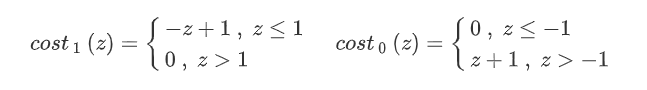
其优化目标和前面提到的logistic分类问题有些相似，具体是：
$$\underset{\theta }{\min }C\sum _{i=1}^m\left[y{}^{\left(i\right)}cost{}_1\left(\theta {}^T{x}^{\left(i\right)}\right)+(1-y{}^{\left(i\right)})cost{}_0\left(\theta {}^{T}x{}^{\left(i\right)}\right)\right]+\frac{1}{2}\sum _{j=1}^n\theta {}_j^2$$

C为调节正则化的参数。

支持向量机和logistic分类不同的是支持向量机只返回0或1（是正样本还是负样本）的结果，并不会返回一个0~1之间的小数来表征概率。因为支持向量机是通过超平面将特征划分为两类的，其中法向量指向的是正类，另一侧为负类。

支持向量机的大边界分类的原理可以简单概括为在满足两个cost函数为0的情况下，最小化后面的正则项，即：

其中，pⁱ为xⁱ在向量θ上的投影。

要使得θ越小，所以p就得越大，由于θ参数是分类超平面的法向量，也就是说每个样本的特征向量在分类超平面的法向量的投影需要越大越好，也就是说每个样本的特征向量和分类超平面的法向量夹角越小越好。如图所示：

为了解决分类中的非线性问题，支持向量机引入了核函数的方法。

由于SVM分类器（未引入核函数之前）的模型是线性的，不能很好的对如下图所示的情况进行分类。所以需要引入核函数来处理非线性的问题。
核函数的解决方案是用新的特征f来代替输入向量的特征x，从而构造新的假设函数：
$$h_{\theta }\left(x\right)={\theta }_1{f}_1+{\theta }_2{f}_2+...+{\theta }_n{f}_n$$
新的特征f如何构造呢？首先我们选取标定向量l，l的选取方法为训练集中每个x的位置。即：
$$l{}^{\left(1\right)}=x{}^{\left(1\right)},l{}^{\left(2\right)}=x{}^{\left(2\right)}...l{}^{\left(n\right)}=x{}^{\left(n\right)}$$

给定一个训练实例x^i，分别对每个l求近似程度来构成新的特征f。求近似程度（f与x/l之间的映射关系）的方法就是我们说的核函数。下面以常用的高斯核函数为例说明其过程：

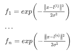
经过以上过程的处理，成功的在假设函数中用f替代了x，接下来的处理过程同上面介绍的线性的SVM。

K-means聚类

K-means是一种聚类算法，属于无监督学习。

可以设置K个聚类中心，也就是将你的训练样本分为K类。算法原理是首先，随机设置K个点，然后将每个训练样本归类到最近的聚类中心，然后将每个聚类中心移动到所以这一类的样本的平均值的位置。重复执行这个过程，直到距离中心不再变化。

需要充分理解K-means算法的损失函数，即：
$$J\left(c{}^{\left(1\right)},...c{}^{\left(m\right)},\mu {}_1,...,{\mu }_K\right)=\frac{1}{m}\sum _{i=1}^m\Vert X{}^{\left(i\right)}-\mu {}_{c{}^{\left(i\right)}}\Vert {}^2$$
其中，cⁱ是指xⁱ所属于是聚类中心，μ是指各个聚类中心的位置。

PCA

PCA （Principal Component Analysis，主成分分析）是一种降维算法。比如需要将三维的数据集降为二维，就是寻找一个离数据点最近的平面，将数据点映射到此平面内。下图为二维数据集降为一维：

PCA算法的数学原理可以参考我的另一篇文章。

异常检测

感觉异常检测算法既可以看做监督学习，又可以看做无监督学习，有点迷。
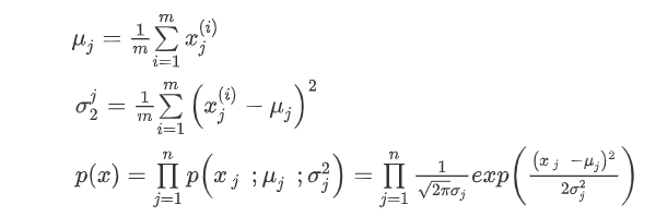
异常分析简单讲就是将数据归一化之后，建立高斯分布模型。然后设置阈值，未能达到阈值的样本就认为是异常样本。
算法具体步骤是对给定数据集，计算每一个维度特征的均值μ和方差σ2。

当$p(x)<\epsilon$时认为是异常。

但是上述算法存在问题，如图所示：

可以通过构建协方差矩阵来解决。当然通过自己根据特征的相关性添加新的组合特征向量也可以解决此问题。

推荐系统

推荐系统是根据用户对已有部分产品的评价来自动的为用户推荐同类产品，从而产生广告效益。（ps：很赚钱）

课程中讲的问题实例是推荐电影。利用已有的各个用户的评分数据去学习下图中？的数据。其中x1，x2可以看做是每个电影的类别信息，x项的多少可以根据情况设定。

采用的方法是协同过滤算法：
$$J\left(x{}^{\left(1\right)},...,x{}^{\left(n_m\right)},\theta {}^{\left(1\right)},...,\theta {}^{\left(n_u\right)}\right)=\frac{1}{2}\sum _{(i,j):r(i,j)=1}\left(\left({\theta }^{\left(j\right)}\right){}^{T}x{}^{\left(i\right)}-y^{\left(i,j\right)}\right){}^2+\frac{\lambda }{2}\sum _{i=1}^{n_m}\sum _{k=1}^n\left(x{}_k^{\left(i\right)}\right){}^2+\frac{\lambda }{2}\sum _{j=1}^{n_u}\sum _{k=1}^n\left(\theta {}_k^{\left(j\right)}\right){}^2$$

算法执行的过程是先对给定的x来优化θ：
$$\underset{\theta {}^{\left(1\right)},...,\theta {}^{\left(nu\right)}}{\min }\frac{1}{2}\sum _{j=1}^{n_u}\sum _{i:r(i,j)=1}\left(\left({\theta }^{\left(j\right)}\right){}^{T}x{}^{\left(i\right)}-y^{\left(i,j\right)}\right){}^2+\frac{\lambda }{2}\sum _{j=1}^{n_u}\sum _{k=1}^n\left(\theta {}_k^{\left(j\right)}\right){}^2$$
让用给定的θ来优化x：
$$\underset{x{}^{\left(1\right)},...,x{}^{\left(n_m\right)}}{\min }\frac{1}{2}\sum _{i=1}^{n_m}\sum _{j:r(i,j)=1}\left(\left({\theta }^{\left(j\right)}\right){}^{T}x{}^{\left(i\right)}-y^{\left(i,j\right)}\right){}^2+\frac{\lambda }{2}\sum _{i=1}^{n_m}\sum _{k=1}^n\left(x{}_k^{\left(i\right)}\right){}^2$$
迭代执行上述两个优化过程，从而实现对总的损失函数J(x,θ)进行优化。