Pointet的读后感(CVPR2016):4分割网络部分

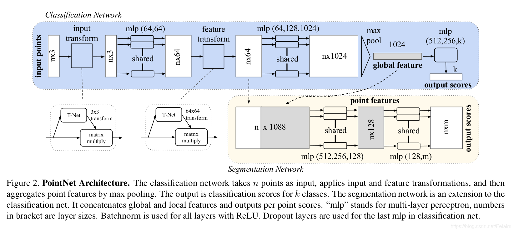
还是先把图放上,分割网络还是相对于分类网络进行修改的,所以看了之前的分类网络的,应该就可以很容易理解分割网络部分了.分割网络先是将分类网络进行旋转归一化后的64维特征取出,再将max_pooling后的1024维特征重复concat到每个点上,相当于给每个点都增加了全局的特征,具体的网络结构如下所示:

def get_model(point_cloud, is_training, bn_decay=None):
    """ ConvNet baseline, input is BxNx3 gray image """
    batch_size = point_cloud.get_shape()[0].value
    num_point = point_cloud.get_shape()[1].value

    input_image = tf.expand_dims(point_cloud, -1)
    # CONV
    net = tf_util.conv2d(input_image, 64, [1, 9], padding='VALID', stride=[1, 1],
                         bn=True, is_training=is_training, scope='conv1', bn_decay=bn_decay)
    net = tf_util.conv2d(net, 64, [1, 1], padding='VALID', stride=[1, 1],
                         bn=True, is_training=is_training, scope='conv2', bn_decay=bn_decay)
    net = tf_util.conv2d(net, 64, [1, 1], padding='VALID', stride=[1, 1],
                         bn=True, is_training=is_training, scope='conv3', bn_decay=bn_decay)
    net = tf_util.conv2d(net, 128, [1, 1], padding='VALID', stride=[1, 1],
                         bn=True, is_training=is_training, scope='conv4', bn_decay=bn_decay)
    points_feat1 = tf_util.conv2d(net, 1024, [1, 1], padding='VALID', stride=[1, 1],
                                  bn=True, is_training=is_training, scope='conv5', bn_decay=bn_decay)
    # MAX
    pc_feat1 = tf_util.max_pool2d(points_feat1, [num_point, 1], padding='VALID', scope='maxpool1')
    # FC
    pc_feat1 = tf.reshape(pc_feat1, [batch_size, -1])
    pc_feat1 = tf_util.fully_connected(pc_feat1, 256, bn=True, is_training=is_training, scope='fc1', bn_decay=bn_decay)
    pc_feat1 = tf_util.fully_connected(pc_feat1, 128, bn=True, is_training=is_training, scope='fc2', bn_decay=bn_decay)
    print(pc_feat1)

    # CONCAT 
    pc_feat1_expand = tf.tile(tf.reshape(pc_feat1, [batch_size, 1, 1, -1]), [1, num_point, 1, 1])
    points_feat1_concat = tf.concat(axis=3, values=[points_feat1, pc_feat1_expand])

    # CONV 
    net = tf_util.conv2d(points_feat1_concat, 512, [1, 1], padding='VALID', stride=[1, 1],
                         bn=True, is_training=is_training, scope='conv6')
    net = tf_util.conv2d(net, 256, [1, 1], padding='VALID', stride=[1, 1],
                         bn=True, is_training=is_training, scope='conv7')
    net = tf_util.dropout(net, keep_prob=0.7, is_training=is_training, scope='dp1')
    net = tf_util.conv2d(net, 13, [1, 1], padding='VALID', stride=[1, 1],
                         activation_fn=None, scope='conv8')
    net = tf.squeeze(net, [2])

    return net

图虽然是这么画的,但是我们可以看到作者给出的网络结构并不是和图片相符合.concat的是升到1024维的特征,和经过max pooling后经过两次全连接层的feature map重复num_point后得到pc_feat1_expand.其实是和原论文放的图是不符的,这边还是需要注意一下的.

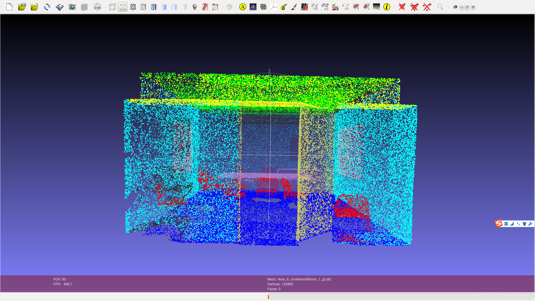
分割网络并不是说和分类网络一样,有具体的训练集和测试集.语义分割网络使用的数据集是Stanford 3D semantic parsing dataset.这个数据有6个area, 271个房间, 总共有13个类别.所以在实际训练中采用的是6折交叉验证的方法,如果LZ想测试area1,那么训练集就是area2一直到area6,如果是area2,那么训练集就是area1, area3-area6,以此类推.

O(∩_∩)O哈哈~要不要看看效果呀?
这个是ground truth…

这个是预测的结果

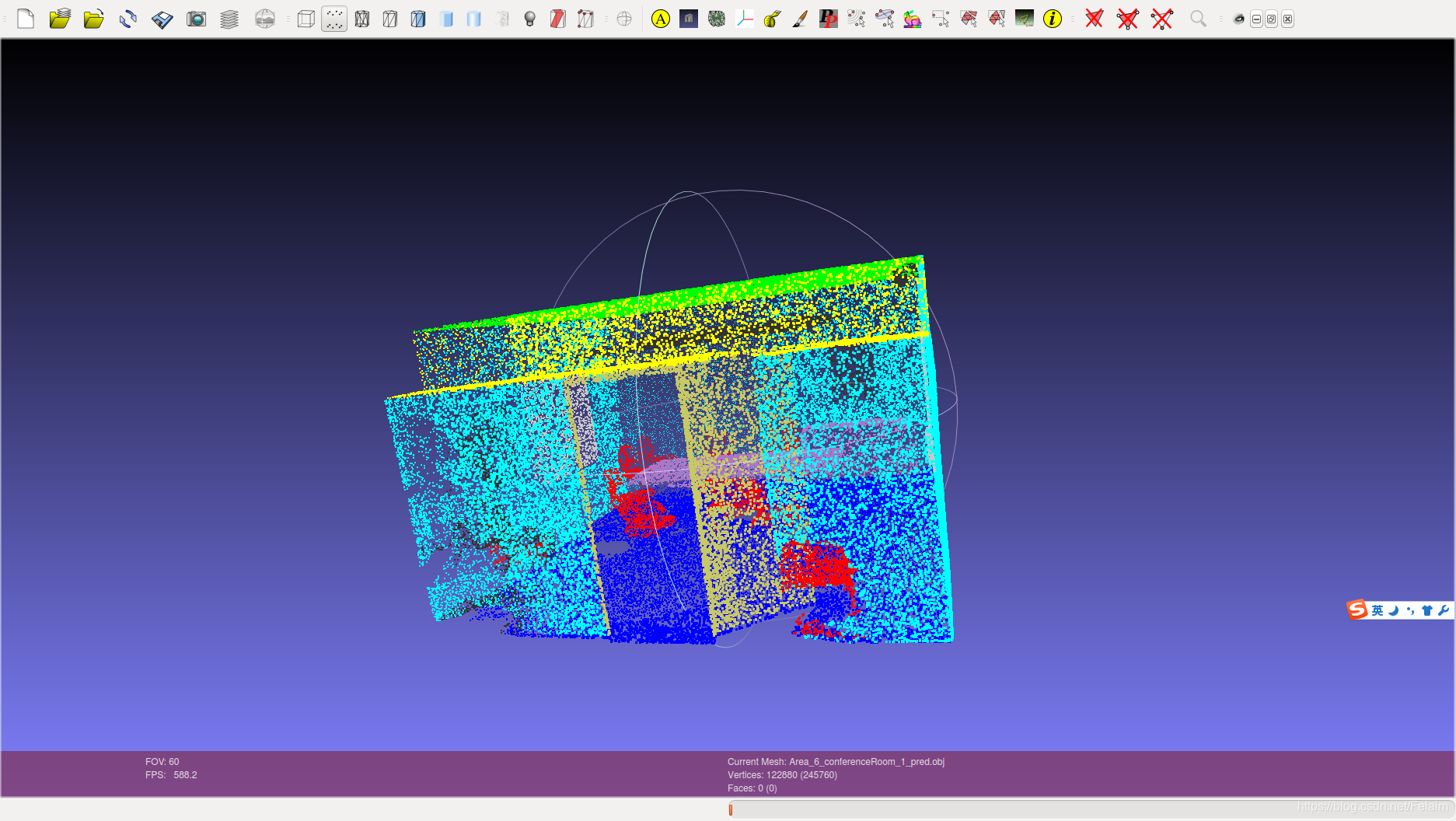
反正效果还是挺好的,从直观上来说…