


Optimization Methods
Until now, you’ve always used Gradient Descent to update the parameters and minimize the cost. In this notebook, you will learn more advanced optimization methods that can speed up learning and perhaps even get you to a better final value for the cost function. Having a good optimization algorithm can be the difference between waiting days vs. just a few hours to get a good result.
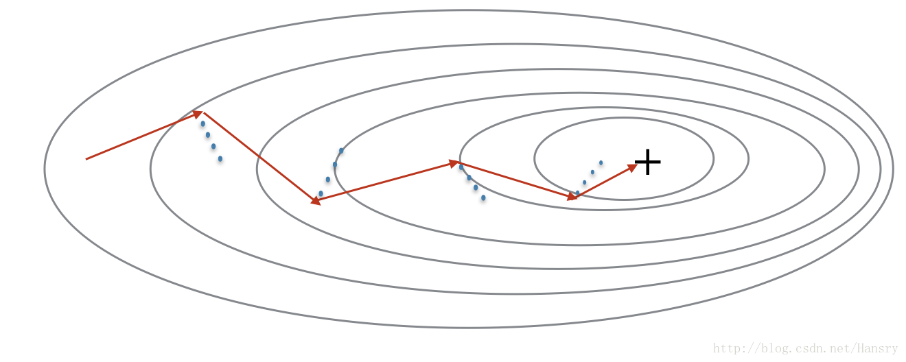
Gradient descent goes “downhill” on a cost function J J J. Think of it as trying to do this:
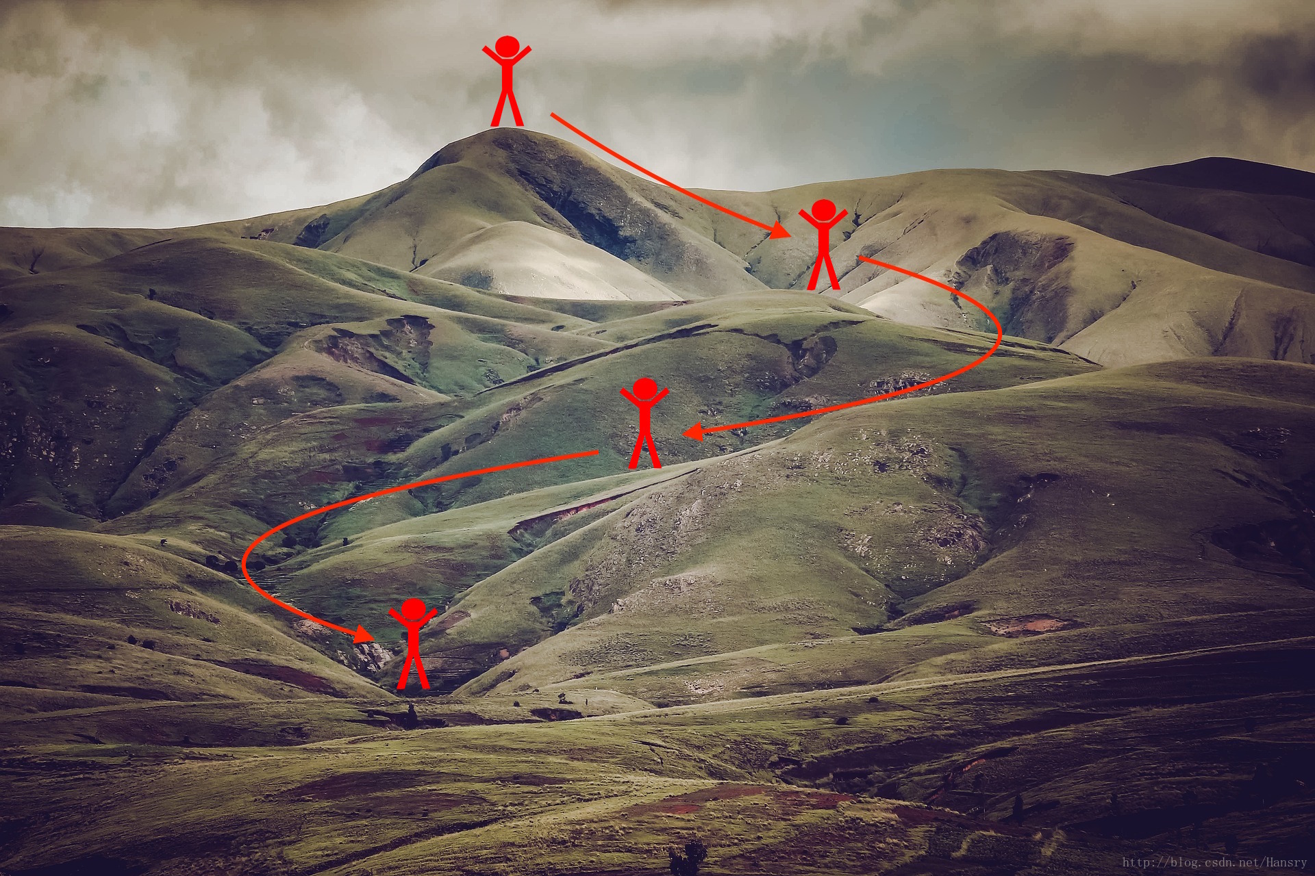
At each step of the training, you update your parameters following a certain direction to try to get to the lowest possible point.
Notations: As usual, $\frac{\partial J}{\partial a } = $ da for any variable a.
To get started, run the following code to import the libraries you will need.
import numpy as np
import matplotlib.pyplot as plt
import scipy.io
import math
import sklearn
import sklearn.datasets

from opt_utils import load_params_and_grads, initialize_parameters, forward_propagation, backward_propagation
from opt_utils import compute_cost, predict, predict_dec, plot_decision_boundary, load_dataset
from testCases import *

plt.rcParams['figure.figsize'] = (7.0, 4.0) # set default size of plots
plt.rcParams['image.interpolation'] = 'nearest'
plt.rcParams['image.cmap'] = 'gray'
opt_utils.py
import numpy as np
import matplotlib.pyplot as plt
import h5py
import scipy.io
import sklearn
import sklearn.datasets

def sigmoid(x):
    """
    Compute the sigmoid of x

    Arguments:
    x -- A scalar or numpy array of any size.

    Return:
    s -- sigmoid(x)
    """
    s = 1/(1+np.exp(-x))
    return s

def relu(x):
    """
    Compute the relu of x

    Arguments:
    x -- A scalar or numpy array of any size.

    Return:
    s -- relu(x)
    """
    s = np.maximum(0,x)

    return s

def load_params_and_grads(seed=1):
    np.random.seed(seed)
    W1 = np.random.randn(2,3)
    b1 = np.random.randn(2,1)
    W2 = np.random.randn(3,3)
    b2 = np.random.randn(3,1)

    dW1 = np.random.randn(2,3)
    db1 = np.random.randn(2,1)
    dW2 = np.random.randn(3,3)
    db2 = np.random.randn(3,1)

    return W1, b1, W2, b2, dW1, db1, dW2, db2


def initialize_parameters(layer_dims):
    """
    Arguments:
    layer_dims -- python array (list) containing the dimensions of each layer in our network

    Returns:
    parameters -- python dictionary containing your parameters "W1", "b1", ..., "WL", "bL":
                    W1 -- weight matrix of shape (layer_dims[l], layer_dims[l-1])
                    b1 -- bias vector of shape (layer_dims[l], 1)
                    Wl -- weight matrix of shape (layer_dims[l-1], layer_dims[l])
                    bl -- bias vector of shape (1, layer_dims[l])

    Tips:
    - For example: the layer_dims for the "Planar Data classification model" would have been [2,2,1].
    This means W1's shape was (2,2), b1 was (1,2), W2 was (2,1) and b2 was (1,1). Now you have to generalize it!
    - In the for loop, use parameters['W' + str(l)] to access Wl, where l is the iterative integer.
    """

    np.random.seed(3)
    parameters = {}
    L = len(layer_dims) # number of layers in the network

    for l in range(1, L):
        parameters['W' + str(l)] = np.random.randn(layer_dims[l], layer_dims[l-1])*  np.sqrt(2.0 / layer_dims[l-1])  #请注意这里的2.0很重要
        parameters['b' + str(l)] = np.zeros((layer_dims[l], 1))

        assert(parameters['W' + str(l)].shape == layer_dims[l], layer_dims[l-1])
        assert(parameters['W' + str(l)].shape == layer_dims[l], 1)

    return parameters


def compute_cost(a3, Y):

    """
    Implement the cost function

    Arguments:
    a3 -- post-activation, output of forward propagation
    Y -- "true" labels vector, same shape as a3

    Returns:
    cost - value of the cost function
    """
    m = Y.shape[1]

    logprobs = np.multiply(-np.log(a3),Y) + np.multiply(-np.log(1 - a3), 1 - Y)
    cost = 1./m * np.sum(logprobs)

    return cost

def forward_propagation(X, parameters):
    """
    Implements the forward propagation (and computes the loss) presented in Figure 2.

    Arguments:
    X -- input dataset, of shape (input size, number of examples)
    parameters -- python dictionary containing your parameters "W1", "b1", "W2", "b2", "W3", "b3":
                    W1 -- weight matrix of shape ()
                    b1 -- bias vector of shape ()
                    W2 -- weight matrix of shape ()
                    b2 -- bias vector of shape ()
                    W3 -- weight matrix of shape ()
                    b3 -- bias vector of shape ()

    Returns:
    loss -- the loss function (vanilla logistic loss)
    """

    # retrieve parameters
    W1 = parameters["W1"]
    b1 = parameters["b1"]
    W2 = parameters["W2"]
    b2 = parameters["b2"]
    W3 = parameters["W3"]
    b3 = parameters["b3"]

    # LINEAR -> RELU -> LINEAR -> RELU -> LINEAR -> SIGMOID
    z1 = np.dot(W1, X) + b1
    a1 = relu(z1)
    z2 = np.dot(W2, a1) + b2
    a2 = relu(z2)
    z3 = np.dot(W3, a2) + b3
    a3 = sigmoid(z3)

    cache = (z1, a1, W1, b1, z2, a2, W2, b2, z3, a3, W3, b3)

    return a3, cache

def backward_propagation(X, Y, cache):
    """
    Implement the backward propagation presented in figure 2.

    Arguments:
    X -- input dataset, of shape (input size, number of examples)
    Y -- true "label" vector (containing 0 if cat, 1 if non-cat)
    cache -- cache output from forward_propagation()

    Returns:
    gradients -- A dictionary with the gradients with respect to each parameter, activation and pre-activation variables
    """
    m = X.shape[1]
    (z1, a1, W1, b1, z2, a2, W2, b2, z3, a3, W3, b3) = cache

    dz3 = 1./m * (a3 - Y)
    dW3 = np.dot(dz3, a2.T)
    db3 = np.sum(dz3, axis=1, keepdims = True)

    da2 = np.dot(W3.T, dz3)
    dz2 = np.multiply(da2, np.int64(a2 > 0))
    dW2 = np.dot(dz2, a1.T)
    db2 = np.sum(dz2, axis=1, keepdims = True)

    da1 = np.dot(W2.T, dz2)
    dz1 = np.multiply(da1, np.int64(a1 > 0))
    dW1 = np.dot(dz1, X.T)
    db1 = np.sum(dz1, axis=1, keepdims = True)

    gradients = {"dz3": dz3, "dW3": dW3, "db3": db3,
                 "da2": da2, "dz2": dz2, "dW2": dW2, "db2": db2,
                 "da1": da1, "dz1": dz1, "dW1": dW1, "db1": db1}

    return gradients

def predict(X, y, parameters):
    """
    This function is used to predict the results of a  n-layer neural network.

    Arguments:
    X -- data set of examples you would like to label
    parameters -- parameters of the trained model

    Returns:
    p -- predictions for the given dataset X
    """

    m = X.shape[1]
    p = np.zeros((1,m), dtype = np.int)

    # Forward propagation
    a3, caches = forward_propagation(X, parameters)

    # convert probas to 0/1 predictions
    for i in range(0, a3.shape[1]):
        if a3[0,i] > 0.5:
            p[0,i] = 1
        else:
            p[0,i] = 0

    # print results

    #print ("predictions: " + str(p[0,:]))
    #print ("true labels: " + str(y[0,:]))
    print("Accuracy: "  + str(np.mean((p[0,:] == y[0,:]))))

    return p

def load_2D_dataset():
    data = scipy.io.loadmat('datasets/data.mat')
    train_X = data['X'].T
    train_Y = data['y'].T
    test_X = data['Xval'].T
    test_Y = data['yval'].T

    plt.scatter(train_X[0, :], train_X[1, :], c=train_Y, s=40, cmap=plt.cm.Spectral);

    return train_X, train_Y, test_X, test_Y

def plot_decision_boundary(model, X, y):
    # Set min and max values and give it some padding
    x_min, x_max = X[0, :].min() - 1, X[0, :].max() + 1
    y_min, y_max = X[1, :].min() - 1, X[1, :].max() + 1
    h = 0.01
    # Generate a grid of points with distance h between them
    xx, yy = np.meshgrid(np.arange(x_min, x_max, h), np.arange(y_min, y_max, h))
    # Predict the function value for the whole grid
    Z = model(np.c_[xx.ravel(), yy.ravel()])
    Z = Z.reshape(xx.shape)
    # Plot the contour and training examples
    plt.contourf(xx, yy, Z, cmap=plt.cm.Spectral)
    plt.ylabel('x2')
    plt.xlabel('x1')
    plt.scatter(X[0, :], X[1, :], c=y, cmap=plt.cm.Spectral)
    plt.show()

def predict_dec(parameters, X):
    """
    Used for plotting decision boundary.

    Arguments:
    parameters -- python dictionary containing your parameters
    X -- input data of size (m, K)

    Returns
    predictions -- vector of predictions of our model (red: 0 / blue: 1)
    """

    # Predict using forward propagation and a classification threshold of 0.5
    a3, cache = forward_propagation(X, parameters)
    predictions = (a3 > 0.5)
    return predictions

def load_dataset():
    np.random.seed(3)
    train_X, train_Y = sklearn.datasets.make_moons(n_samples=300, noise=.2) #300 #0.2
    # Visualize the data
    plt.scatter(train_X[:, 0], train_X[:, 1], c=train_Y, s=40, cmap=plt.cm.Spectral);
    train_X = train_X.T
    train_Y = train_Y.reshape((1, train_Y.shape[0]))

    return train_X, train_Y
1 - Gradient Descent
A simple optimization method in machine learning is gradient descent (GD). When you take gradient steps with respect to all m m m examples on each step, it is also called Batch Gradient Descent.
Warm-up exercise: Implement the gradient descent update rule. The gradient descent rule is, for
l
=
1
,
.
.
.
,
L
l = 1, ..., L
l=1,...,L:
(1)
W
[
l
]
=
W
[
l
]
−
α
d
W
[
l
]
W^{[l]} = W^{[l]} - \alpha \text{ } dW^{[l]} \tag{1}
W[l]=W[l]−α dW[l](1)
(2)
b
[
l
]
=
b
[
l
]
−
α
d
b
[
l
]
b^{[l]} = b^{[l]} - \alpha \text{ } db^{[l]} \tag{2}
b[l]=b[l]−α db[l](2)
where L is the number of layers and
α
\alpha
α is the learning rate. All parameters should be stored in the parameters dictionary. Note that the iterator l starts at 0 in the for loop while the first parameters are
W
[
1
]
W^{[1]}
W[1] and
b
[
1
]
b^{[1]}
b[1]. You need to shift l to l+1 when coding.
def update_parameters_with_gd(parameters, grads, learning_rate):
    """
    Update parameters using one step of gradient descent

    Arguments:
    parameters -- python dictionary containing your parameters to be updated:
                    parameters['W' + str(l)] = Wl
                    parameters['b' + str(l)] = bl
    grads -- python dictionary containing your gradients to update each parameters:
                    grads['dW' + str(l)] = dWl
                    grads['db' + str(l)] = dbl
    learning_rate -- the learning rate, scalar.

    Returns:
    parameters -- python dictionary containing your updated parameters
    """

    L = len(parameters) // 2 # number of layers in the neural networks

    # Update rule for each parameter
    for l in range(L):
        ### START CODE HERE ### (approx. 2 lines)
        parameters["W" + str(l+1)] = parameters["W"+str(l+1)]-learning_rate*grads["dW"+str(l+1)]
        parameters["b" + str(l+1)] = parameters["b"+str(l+1)]-learning_rate*grads["db"+str(l+1)]
        ### END CODE HERE ###

    return parameters
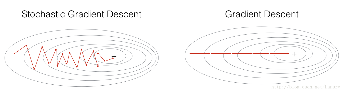
A variant of this is Stochastic Gradient Descent (SGD), which is equivalent to mini-batch gradient descent where each mini-batch has just 1 example. The update rule that you have just implemented does not change. What changes is that you would be computing gradients on just one training example at a time, rather than on the whole training set. The code examples below illustrate the difference between stochastic gradient descent and (batch) gradient descent.
- (Batch) Gradient Descent:
X = data_input
Y = labels
parameters = initialize_parameters(layers_dims)
for i in range(0, num_iterations):
    # Forward propagation
    a, caches = forward_propagation(X, parameters)
    # Compute cost.
    cost = compute_cost(a, Y)
    # Backward propagation.
    grads = backward_propagation(a, caches, parameters)
    # Update parameters.
    parameters = update_parameters(parameters, grads)
- Stochastic Gradient Descent:
X = data_input
Y = labels
parameters = initialize_parameters(layers_dims)
for i in range(0, num_iterations):
    for j in range(0, m):
        # Forward propagation
        a, caches = forward_propagation(X[:,j], parameters)
        # Compute cost
        cost = compute_cost(a, Y[:,j])
        # Backward propagation
        grads = backward_propagation(a, caches, parameters)
        # Update parameters.
        parameters = update_parameters(parameters, grads)
In Stochastic Gradient Descent, you use only 1 training example before updating the gradients. When the training set is large, SGD can be faster. But the parameters will “oscillate” toward the minimum rather than converge smoothly. Here is an illustration of this:
Note also that implementing SGD requires 3 for-loops in total:
- Over the number of iterations
- Over the m m m training examples
- Over the layers (to update all parameters, from ( W [ 1 ] , b [ 1 ] ) (W^{[1]},b^{[1]}) (W[1],b[1]) to ( W [ L ] , b [ L ] ) (W^{[L]},b^{[L]}) (W[L],b[L]))
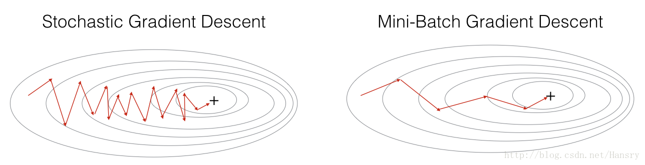
In practice, you’ll often get faster results if you do not use neither the whole training set, nor only one training example, to perform each update. Mini-batch gradient descent uses an intermediate number of examples for each step. With mini-batch gradient descent, you loop over the mini-batches instead of looping over individual training examples.
What you should remember:
- The difference between gradient descent, mini-batch gradient descent and stochastic gradient descent is the number of examples you use to perform one update step.
- You have to tune a learning rate hyperparameter α \alpha α.
- With a well-turned mini-batch size, usually it outperforms either gradient descent or stochastic gradient descent (particularly when the training set is large).
2 - Mini-Batch Gradient descent
Let’s learn how to build mini-batches from the training set (X, Y).
There are two steps:
-
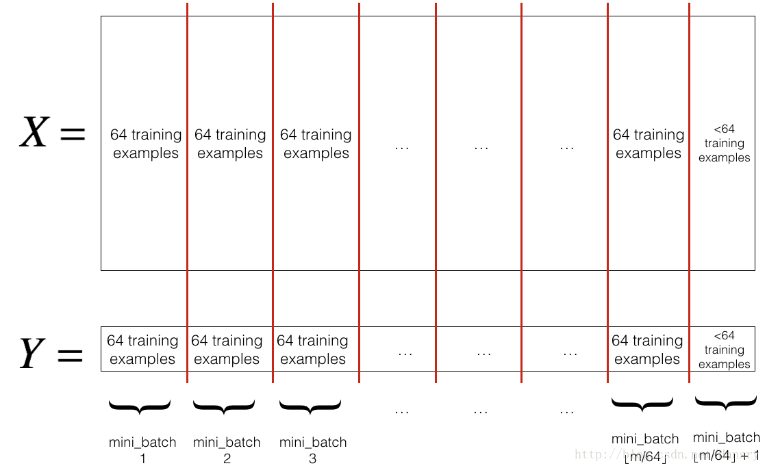
Shuffle: Create a shuffled version of the training set (X, Y) as shown below. Each column of X and Y represents a training example. Note that the random shuffling is done synchronously between X and Y. Such that after the shuffling the i t h i^{th} ith column of X is the example corresponding to the i t h i^{th} ith label in Y. The shuffling step ensures that examples will be split randomly into different mini-batches.
-
Partition: Partition the shuffled (X, Y) into mini-batches of size
mini_batch_size(here 64). Note that the number of training examples is not always divisible bymini_batch_size. The last mini batch might be smaller, but you don’t need to worry about this. When the final mini-batch is smaller than the fullmini_batch_size, it will look like this:
Exercise: Implement random_mini_batches. We coded the shuffling part for you. To help you with the partitioning step, we give you the following code that selects the indexes for the
1
s
t
1^{st}
1st and
2
n
d
2^{nd}
2nd mini-batches:
first_mini_batch_X = shuffled_X[:, 0 : mini_batch_size]
second_mini_batch_X = shuffled_X[:, mini_batch_size : 2 * mini_batch_size]
...
Note that the last mini-batch might end up smaller than mini_batch_size=64. Let
⌊
s
⌋
\lfloor s \rfloor
⌊s⌋ represents
s
s
s rounded down to the nearest integer (this is math.floor(s) in Python). If the total number of examples is not a multiple of mini_batch_size=64 then there will be
⌊
m
m
i
n
i
_
b
a
t
c
h
_
s
i
z
e
⌋
\lfloor \frac{m}{mini\_batch\_size}\rfloor
⌊mini_batch_sizem⌋ mini-batches with a full 64 examples, and the number of examples in the final mini-batch will be (
m
−
m
i
n
i
_
b
a
t
c
h
_
s
i
z
e
×
⌊
m
m
i
n
i
_
b
a
t
c
h
_
s
i
z
e
⌋
m-mini_\_batch_\_size \times \lfloor \frac{m}{mini\_batch\_size}\rfloor
m−mini_batch_size×⌊mini_batch_sizem⌋).
def random_mini_batches(X, Y, mini_batch_size = 64, seed = 0):
    """
    Creates a list of random minibatches from (X, Y)

    Arguments:
    X -- input data, of shape (input size, number of examples)
    Y -- true "label" vector (1 for blue dot / 0 for red dot), of shape (1, number of examples)
    mini_batch_size -- size of the mini-batches, integer

    Returns:
    mini_batches -- list of synchronous (mini_batch_X, mini_batch_Y)
    """

    np.random.seed(seed)            # To make your "random" minibatches the same as ours
    m = X.shape[1]                  # number of training examples
    mini_batches = []

    # Step 1: Shuffle (X, Y)
    permutation = list(np.random.permutation(m))
    shuffled_X = X[:, permutation]
    shuffled_Y = Y[:, permutation].reshape((1,m))

    # Step 2: Partition (shuffled_X, shuffled_Y). Minus the end case.
    num_complete_minibatches = math.floor(m/mini_batch_size) # number of mini batches of size mini_batch_size in your partitionning
    for k in range(0, num_complete_minibatches):
        ### START CODE HERE ### (approx. 2 lines)
        mini_batch_X = shuffled_X[:,k*mini_batch_size:(k+1)*mini_batch_size]
        mini_batch_Y = shuffled_Y[:,k*mini_batch_size:(k+1)*mini_batch_size]
        ### END CODE HERE ###
        mini_batch = (mini_batch_X, mini_batch_Y)
        mini_batches.append(mini_batch)

    # Handling the end case (last mini-batch < mini_batch_size)
    if m % mini_batch_size != 0:
        ### START CODE HERE ### (approx. 2 lines)
        mini_batch_X = shuffled_X[:,mini_batch_size*num_complete_minibatches:]
        mini_batch_Y = shuffled_Y[:,mini_batch_size*num_complete_minibatches:]
        ### END CODE HERE ###
        mini_batch = (mini_batch_X, mini_batch_Y)
        mini_batches.append(mini_batch)

    return mini_batches
3 - Momentum
Because mini-batch gradient descent makes a parameter update after seeing just a subset of examples, the direction of the update has some variance, and so the path taken by mini-batch gradient descent will “oscillate” toward convergence. Using momentum can reduce these oscillations.
Momentum takes into account the past gradients to smooth out the update. We will store the ‘direction’ of the previous gradients in the variable v v v. Formally, this will be the exponentially weighted average of the gradient on previous steps. You can also think of v v v as the “velocity” of a ball rolling downhill, building up speed (and momentum) according to the direction of the gradient/slope of the hill.
Exercise: Initialize the velocity. The velocity,
v
v
v, is a python dictionary that needs to be initialized with arrays of zeros. Its keys are the same as those in the grads dictionary, that is:
for
l
=
1
,
.
.
.
,
L
l =1,...,L
l=1,...,L:
v["dW" + str(l+1)] = ... #(numpy array of zeros with the same shape as parameters["W" + str(l+1)])
v["db" + str(l+1)] = ... #(numpy array of zeros with the same shape as parameters["b" + str(l+1)])
Note that the iterator l starts at 0 in the for loop while the first parameters are v[“dW1”] and v[“db1”] (that’s a “one” on the superscript). This is why we are shifting l to l+1 in the for loop.
def initialize_velocity(parameters):
    """
    Initializes the velocity as a python dictionary with:
                - keys: "dW1", "db1", ..., "dWL", "dbL"
                - values: numpy arrays of zeros of the same shape as the corresponding gradients/parameters.
    Arguments:
    parameters -- python dictionary containing your parameters.
                    parameters['W' + str(l)] = Wl
                    parameters['b' + str(l)] = bl

    Returns:
    v -- python dictionary containing the current velocity.
                    v['dW' + str(l)] = velocity of dWl
                    v['db' + str(l)] = velocity of dbl
    """

    L = len(parameters) // 2 # number of layers in the neural networks
    v = {}

    # Initialize velocity
    for l in range(L):
        ### START CODE HERE ### (approx. 2 lines)
        v["dW" + str(l+1)] = np.zeros(parameters["W"+str(l+1)].shape)
        v["db" + str(l+1)] = np.zeros(parameters["b"+str(l+1)].shape)
        ### END CODE HERE ###

    return v
def update_parameters_with_momentum(parameters, grads, v, beta, learning_rate):
    """
    Update parameters using Momentum

    Arguments:
    parameters -- python dictionary containing your parameters:
                    parameters['W' + str(l)] = Wl
                    parameters['b' + str(l)] = bl
    grads -- python dictionary containing your gradients for each parameters:
                    grads['dW' + str(l)] = dWl
                    grads['db' + str(l)] = dbl
    v -- python dictionary containing the current velocity:
                    v['dW' + str(l)] = ...
                    v['db' + str(l)] = ...
    beta -- the momentum hyperparameter, scalar
    learning_rate -- the learning rate, scalar

    Returns:
    parameters -- python dictionary containing your updated parameters
    v -- python dictionary containing your updated velocities
    """

    L = len(parameters) // 2 # number of layers in the neural networks

    # Momentum update for each parameter
    for l in range(L):

        ### START CODE HERE ### (approx. 4 lines)
        # compute velocities
        v["dW" + str(l+1)] = beta*v["dW"+str(l+1)]+(1-beta)*grads["dW"+str(l+1)]
        v["db" + str(l+1)] = beta*v["db"+str(l+1)]+(1-beta)*grads["db"+str(l+1)]
        # update parameters
        parameters["W" + str(l+1)] = parameters["W"+str(l+1)] - v["dW"+str(l+1)]*learning_rate
        parameters["b" + str(l+1)] = parameters["b"+str(l+1)] -v["db"+str(l+1)]*learning_rate
        ### END CODE HERE ###

    return parameters, v
4 - Adam
Adam is one of the most effective optimization algorithms for training neural networks. It combines ideas from RMSProp (described in lecture) and Momentum.
How does Adam work?
- It calculates an exponentially weighted average of past gradients, and stores it in variables v v v (before bias correction) and v c o r r e c t e d v^{corrected} vcorrected (with bias correction).
- It calculates an exponentially weighted average of the squares of the past gradients, and stores it in variables s s s (before bias correction) and s c o r r e c t e d s^{corrected} scorrected (with bias correction).
- It updates parameters in a direction based on combining information from “1” and “2”.
The update rule is, for l = 1 , . . . , L l = 1, ..., L l=1,...,L:
{
v
d
W
[
l
]
=
β
1
v
d
W
[
l
]
+
(
1
−
β
1
)
∂
J
∂
W
[
l
]
v
d
W
[
l
]
c
o
r
r
e
c
t
e
d
=
v
d
W
[
l
]
1
−
(
β
1
)
t
s
d
W
[
l
]
=
β
2
s
d
W
[
l
]
+
(
1
−
β
2
)
(
∂
J
∂
W
[
l
]
)
2
s
d
W
[
l
]
c
o
r
r
e
c
t
e
d
=
s
d
W
[
l
]
1
−
(
β
1
)
t
W
[
l
]
=
W
[
l
]
−
α
v
d
W
[
l
]
c
o
r
r
e
c
t
e
d
s
d
W
[
l
]
c
o
r
r
e
c
t
e
d
+
ε
\begin{cases} v_{dW^{[l]}} = \beta_1 v_{dW^{[l]}} + (1 - \beta_1) \frac{\partial \mathcal{J} }{ \partial W^{[l]} } \\ v^{corrected}_{dW^{[l]}} = \frac{v_{dW^{[l]}}}{1 - (\beta_1)^t} \\ s_{dW^{[l]}} = \beta_2 s_{dW^{[l]}} + (1 - \beta_2) (\frac{\partial \mathcal{J} }{\partial W^{[l]} })^2 \\ s^{corrected}_{dW^{[l]}} = \frac{s_{dW^{[l]}}}{1 - (\beta_1)^t} \\ W^{[l]} = W^{[l]} - \alpha \frac{v^{corrected}_{dW^{[l]}}}{\sqrt{s^{corrected}_{dW^{[l]}}} + \varepsilon} \end{cases}
⎩⎪⎪⎪⎪⎪⎪⎪⎪⎨⎪⎪⎪⎪⎪⎪⎪⎪⎧vdW[l]=β1vdW[l]+(1−β1)∂W[l]∂JvdW[l]corrected=1−(β1)tvdW[l]sdW[l]=β2sdW[l]+(1−β2)(∂W[l]∂J)2sdW[l]corrected=1−(β1)tsdW[l]W[l]=W[l]−αsdW[l]corrected+εvdW[l]corrected
where:
- t counts the number of steps taken of Adam
- L is the number of layers
- β 1 \beta_1 β1 and β 2 \beta_2 β2 are hyperparameters that control the two exponentially weighted averages.
- α \alpha α is the learning rate
- ε \varepsilon ε is a very small number to avoid dividing by zero
As usual, we will store all parameters in the parameters dictionary
Exercise: Initialize the Adam variables
v
,
s
v, s
v,s which keep track of the past information.
Instruction: The variables
v
,
s
v, s
v,s are python dictionaries that need to be initialized with arrays of zeros. Their keys are the same as for grads, that is:
for
l
=
1
,
.
.
.
,
L
l = 1, ..., L
l=1,...,L:
v["dW" + str(l+1)] = ... #(numpy array of zeros with the same shape as parameters["W" + str(l+1)])
v["db" + str(l+1)] = ... #(numpy array of zeros with the same shape as parameters["b" + str(l+1)])
s["dW" + str(l+1)] = ... #(numpy array of zeros with the same shape as parameters["W" + str(l+1)])
s["db" + str(l+1)] = ... #(numpy array of zeros with the same shape as parameters["b" + str(l+1)])
def initialize_adam(parameters) :
    """
    Initializes v and s as two python dictionaries with:
                - keys: "dW1", "db1", ..., "dWL", "dbL"
                - values: numpy arrays of zeros of the same shape as the corresponding gradients/parameters.

    Arguments:
    parameters -- python dictionary containing your parameters.
                    parameters["W" + str(l)] = Wl
                    parameters["b" + str(l)] = bl

    Returns:
    v -- python dictionary that will contain the exponentially weighted average of the gradient.
                    v["dW" + str(l)] = ...
                    v["db" + str(l)] = ...
    s -- python dictionary that will contain the exponentially weighted average of the squared gradient.
                    s["dW" + str(l)] = ...
                    s["db" + str(l)] = ...

    """

    L = len(parameters) // 2 # number of layers in the neural networks
    v = {}
    s = {}

    # Initialize v, s. Input: "parameters". Outputs: "v, s".
    for l in range(L):
    ### START CODE HERE ### (approx. 4 lines)
        v["dW" + str(l+1)] = np.zeros(parameters["W"+str(l+1)].shape)
        v["db" + str(l+1)] = np.zeros(parameters["b"+str(l+1)].shape)
        s["dW" + str(l+1)] = np.zeros(parameters["W"+str(l+1)].shape)
        s["db" + str(l+1)] = np.zeros(parameters["b"+str(l+1)].shape)
    ### END CODE HERE ###

    return v, s
def update_parameters_with_adam(parameters, grads, v, s, t, learning_rate = 0.01,
                                beta1 = 0.9, beta2 = 0.999,  epsilon = 1e-8):
    """
    Update parameters using Adam

    Arguments:
    parameters -- python dictionary containing your parameters:
                    parameters['W' + str(l)] = Wl
                    parameters['b' + str(l)] = bl
    grads -- python dictionary containing your gradients for each parameters:
                    grads['dW' + str(l)] = dWl
                    grads['db' + str(l)] = dbl
    v -- Adam variable, moving average of the first gradient, python dictionary
    s -- Adam variable, moving average of the squared gradient, python dictionary
    learning_rate -- the learning rate, scalar.
    beta1 -- Exponential decay hyperparameter for the first moment estimates
    beta2 -- Exponential decay hyperparameter for the second moment estimates
    epsilon -- hyperparameter preventing division by zero in Adam updates

    Returns:
    parameters -- python dictionary containing your updated parameters
    v -- Adam variable, moving average of the first gradient, python dictionary
    s -- Adam variable, moving average of the squared gradient, python dictionary
    """

    L = len(parameters) // 2                 # number of layers in the neural networks
    v_corrected = {}                         # Initializing first moment estimate, python dictionary
    s_corrected = {}                         # Initializing second moment estimate, python dictionary

    # Perform Adam update on all parameters
    for l in range(L):
        # Moving average of the gradients. Inputs: "v, grads, beta1". Output: "v".
        ### START CODE HERE ### (approx. 2 lines)
        v["dW" + str(l+1)] = beta1*v["dW"+str(l+1)]+(1-beta1)*grads["dW"+str(l+1)]
        v["db" + str(l+1)] = beta1*v["db"+str(l+1)]+(1-beta1)*grads["db"+str(l+1)]
        ### END CODE HERE ###

        # Compute bias-corrected first moment estimate. Inputs: "v, beta1, t". Output: "v_corrected".
        ### START CODE HERE ### (approx. 2 lines)
        v_corrected["dW" + str(l+1)] = v["dW"+str(l+1)]/(1-beta1**t)
        v_corrected["db" + str(l+1)] = v["db"+str(l+1)]/(1-beta1**t)
        ### END CODE HERE ###

        # Moving average of the squared gradients. Inputs: "s, grads, beta2". Output: "s".
        ### START CODE HERE ### (approx. 2 lines)
        s["dW" + str(l+1)] = beta2*s["dW"+str(l+1)]+(1-beta2)*np.power(grads["dW"+str(l+1)],2)
        s["db" + str(l+1)] = beta2*s["db"+str(l+1)]+(1-beta2)*np.power(grads["db"+str(l+1)],2)
        ### END CODE HERE ###

        # Compute bias-corrected second raw moment estimate. Inputs: "s, beta2, t". Output: "s_corrected".
        ### START CODE HERE ### (approx. 2 lines)
        s_corrected["dW" + str(l+1)] = s["dW"+str(l+1)]/(1-beta2**t)
        s_corrected["db" + str(l+1)] = s["db"+str(l+1)]/(1-beta2**t)
        ### END CODE HERE ###

        # Update parameters. Inputs: "parameters, learning_rate, v_corrected, s_corrected, epsilon". Output: "parameters".
        ### START CODE HERE ### (approx. 2 lines)
        parameters["W" + str(l+1)] = parameters["W"+str(l+1)]-learning_rate*v_corrected["dW"+str(l+1)]/(np.sqrt(s_corrected["dW"+str(l+1)])+epsilon)
        parameters["b" + str(l+1)] = parameters["b"+str(l+1)]-learning_rate*v_corrected["db"+str(l+1)]/(np.sqrt(s_corrected["db"+str(l+1)])+epsilon)
        ### END CODE HERE ###

    return parameters, v, s
5 - Model with different optimization algorithms
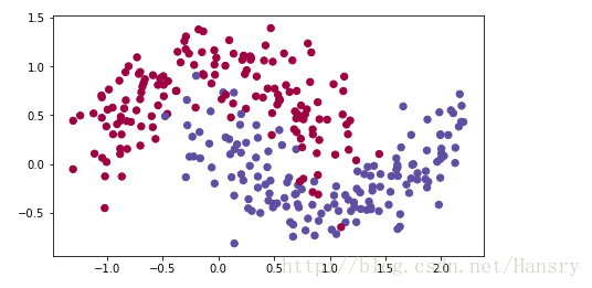
Lets use the following “moons” dataset to test the different optimization methods. (The dataset is named “moons” because the data from each of the two classes looks a bit like a crescent-shaped moon.)
train_X, train_Y = load_dataset()
We have already implemented a 3-layer neural network. You will train it with:
- Mini-batch Gradient Descent: it will call your function:
update_parameters_with_gd()
- Mini-batch Momentum: it will call your functions:
initialize_velocity()andupdate_parameters_with_momentum()
- Mini-batch Adam: it will call your functions:
initialize_adam()andupdate_parameters_with_adam()
def model(X, Y, layers_dims, optimizer, learning_rate = 0.0007, mini_batch_size = 64, beta = 0.9,
          beta1 = 0.9, beta2 = 0.999,  epsilon = 1e-8, num_epochs = 10000, print_cost = True):
    """
    3-layer neural network model which can be run in different optimizer modes.

    Arguments:
    X -- input data, of shape (2, number of examples)
    Y -- true "label" vector (1 for blue dot / 0 for red dot), of shape (1, number of examples)
    layers_dims -- python list, containing the size of each layer
    learning_rate -- the learning rate, scalar.
    mini_batch_size -- the size of a mini batch
    beta -- Momentum hyperparameter
    beta1 -- Exponential decay hyperparameter for the past gradients estimates
    beta2 -- Exponential decay hyperparameter for the past squared gradients estimates
    epsilon -- hyperparameter preventing division by zero in Adam updates
    num_epochs -- number of epochs
    print_cost -- True to print the cost every 1000 epochs

    Returns:
    parameters -- python dictionary containing your updated parameters
    """

    L = len(layers_dims)             # number of layers in the neural networks
    costs = []                       # to keep track of the cost
    t = 0                            # initializing the counter required for Adam update
    seed = 10                        # For grading purposes, so that your "random" minibatches are the same as ours

    # Initialize parameters
    parameters = initialize_parameters(layers_dims)

    # Initialize the optimizer
    if optimizer == "gd":
        pass # no initialization required for gradient descent
    elif optimizer == "momentum":
        v = initialize_velocity(parameters)
    elif optimizer == "adam":
        v, s = initialize_adam(parameters)

    # Optimization loop
    for i in range(num_epochs):

        # Define the random minibatches. We increment the seed to reshuffle differently the dataset after each epoch
        seed = seed + 1
        minibatches = random_mini_batches(X, Y, mini_batch_size, seed)

        for minibatch in minibatches:

            # Select a minibatch
            (minibatch_X, minibatch_Y) = minibatch

            # Forward propagation
            a3, caches = forward_propagation(minibatch_X, parameters)

            # Compute cost
            cost = compute_cost(a3, minibatch_Y)

            # Backward propagation
            grads = backward_propagation(minibatch_X, minibatch_Y, caches)

            # Update parameters
            if optimizer == "gd":
                parameters = update_parameters_with_gd(parameters, grads, learning_rate)
            elif optimizer == "momentum":
                parameters, v = update_parameters_with_momentum(parameters, grads, v, beta, learning_rate)
            elif optimizer == "adam":
                t = t + 1 # Adam counter
                parameters, v, s = update_parameters_with_adam(parameters, grads, v, s,
                                                               t, learning_rate, beta1, beta2,  epsilon)

        # Print the cost every 1000 epoch
        if print_cost and i % 1000 == 0:
            print ("Cost after epoch %i: %f" %(i, cost))
        if print_cost and i % 100 == 0:
            costs.append(cost)

    # plot the cost
    plt.plot(costs)
    plt.ylabel('cost')
    plt.xlabel('epochs (per 100)')
    plt.title("Learning rate = " + str(learning_rate))
    plt.show()

    return parameters
You will now run this 3 layer neural network with each of the 3 optimization methods.
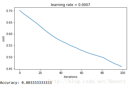
5.1 - Mini-batch Gradient descent
Run the following code to see how the model does with mini-batch gradient descent.
layers_dims = [train_X.shape[0], 5, 2, 1]
parameters = model(train_X, train_Y, layers_dims, optimizer = "gd")

# Predict
predictions = predict(train_X, train_Y, parameters)

# Plot decision boundary
plt.title("Model with Gradient Descent optimization")
axes = plt.gca()
axes.set_xlim([-1.5,2.5])
axes.set_ylim([-1,1.5])
plot_decision_boundary(lambda x: predict_dec(parameters, x.T), train_X, train_Y)
cost after epochs 0 is: 0.701125719795
cost after epochs 1000 is: 0.666807551123
cost after epochs 2000 is: 0.632183197071
cost after epochs 3000 is: 0.596733513902
cost after epochs 4000 is: 0.569728695966
cost after epochs 5000 is: 0.548034534678
cost after epochs 6000 is: 0.528443224165
cost after epochs 7000 is: 0.512129543319
cost after epochs 8000 is: 0.498509846698
cost after epochs 9000 is: 0.47573828208
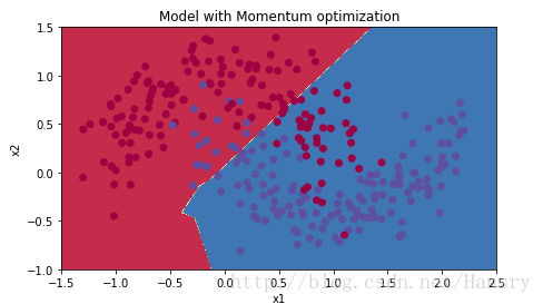
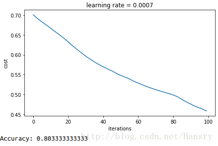
5.2 - Mini-batch gradient descent with momentum
Run the following code to see how the model does with momentum. Because this example is relatively simple, the gains from using momemtum are small; but for more complex problems you might see bigger gains.
# train 3-layer model
layers_dims = [train_X.shape[0], 5, 2, 1]
parameters = model(train_X, train_Y, layers_dims, beta = 0.9, optimizer = "momentum")
# Predict
predictions = predict(train_X, train_Y, parameters)
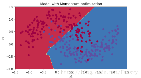
# Plot decision boundary
plt.title("Model with Momentum optimization")
axes = plt.gca()
axes.set_xlim([-1.5,2.5])
axes.set_ylim([-1,1.5])
plot_decision_boundary(lambda x: predict_dec(parameters, x.T), train_X, train_Y)
cost after epochs 0 is: 0.701125719795
cost after epochs 1000 is: 0.666807551123
cost after epochs 2000 is: 0.632183197071
cost after epochs 3000 is: 0.596733513902
cost after epochs 4000 is: 0.569728695966
cost after epochs 5000 is: 0.548034534678
cost after epochs 6000 is: 0.528443224165
cost after epochs 7000 is: 0.512129543319
cost after epochs 8000 is: 0.498509846698
cost after epochs 9000 is: 0.47573828208
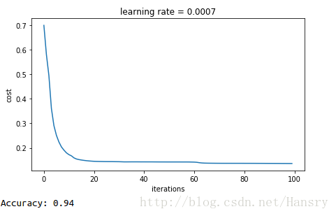
5.3 - Mini-batch with Adam mode
Run the following code to see how the model does with Adam.
layers_dims = [train_X.shape[0], 5, 2, 1]
parameters = model(train_X, train_Y, layers_dims, optimizer = "adam")
# Predict
predictions = predict(train_X, train_Y, parameters)
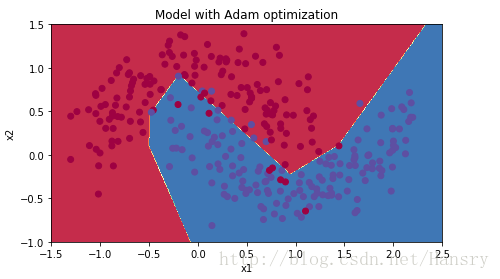
# Plot decision boundary
plt.title("Model with Adam optimization")
axes = plt.gca()
axes.set_xlim([-1.5,2.5])
axes.set_ylim([-1,1.5])
plot_decision_boundary(lambda x: predict_dec(parameters, x.T), train_X, train_Y)
cost after epochs 0 is: 0.700275600301
cost after epochs 1000 is: 0.17229901058
cost after epochs 2000 is: 0.145090465993
cost after epochs 3000 is: 0.143431884902
cost after epochs 4000 is: 0.142750195505
cost after epochs 5000 is: 0.142411457077
cost after epochs 6000 is: 0.141755681408
cost after epochs 7000 is: 0.137016078743
cost after epochs 8000 is: 0.136850127175
cost after epochs 9000 is: 0.136540429643
5.4 - Summary
</tr>
    <td>
    Gradient descent
    </td>
    <td>
    80.33%
    </td>
    <td>
    oscillations
    </td>
<tr>
    <td>
    Momentum
    </td>
    <td>
    80.33%
    </td>
    <td>
    oscillations
    </td>
</tr>
<tr>
    <td>
    Adam
    </td>
    <td>
    94%
    </td>
    <td>
    smoother
    </td>
</tr>
| **optimization method** | **accuracy** | **cost shape** |
Momentum usually helps, but given the small learning rate and the simplistic dataset, its impact is almost negligeable. Also, the huge oscillations you see in the cost come from the fact that some minibatches are more difficult thans others for the optimization algorithm.
Adam on the other hand, clearly outperforms mini-batch gradient descent and Momentum. If you run the model for more epochs on this simple dataset, all three methods will lead to very good results. However, you’ve seen that Adam converges a lot faster.
Some advantages of Adam include:
- Relatively low memory requirements (though higher than gradient descent and gradient descent with momentum)
- Usually works well even with little tuning of hyperparameters (except α \alpha α)
Tip: 当你程序一直迭代但是cost却不变的时候,请注意检查你的初始parameters,“2” 与“ 2.0”有时候真的会是导致你算法出错的关键地方


 662
662


 被折叠的 条评论
为什么被折叠?
被折叠的 条评论
为什么被折叠?
 到【灌水乐园】发言


