TensorFlow + Keras 图像识别：Dogs vs Cats Image Classification with data augmentation(CNN, 解决过拟合问题)

最新推荐文章于 2023-11-26 10:14:14 发布

一念逍遥、

最新推荐文章于 2023-11-26 10:14:14 发布

阅读量1.8k

点赞数 2

分类专栏： tensorflow 文章标签： TensorFlow Keras 神经网络 CNN

本文链接：https://blog.csdn.net/Happy_hui520/article/details/95474814

版权

tensorflow 同时被 2 个专栏收录

5 篇文章 0 订阅

订阅专栏

神经网络

5 篇文章 0 订阅

订阅专栏

OS：Win10

Interpreter: Python3.7

Environment: Anaconda3 + Tensorflow-gpu2.0.0 + Spyder

API: tf.keras(a high-level API to build and train models in TensorFlow)

项目源码参考自TensorFlow官方教程https://colab.research.google.com/github/tensorflow/examples/blob/master/courses/udacity_intro_to_tensorflow_for_deep_learning/l05c02_dogs_vs_cats_with_augmentation.ipynb

项目简介

在这篇教程中，我们将讨论如何对猫或狗的图片进行分类。我们将使用tf.keras.Sequential构建一个CNN图像分类器，使用 tf.keras.preprocessing.image.ImageDataGenerator类来加载数据。

我们用的是 Dogs vs. Cats dataset ，数据集的详细介绍请看官网： https://www.kaggle.com/c/dogs-vs-cats/data

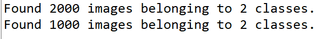
数据集包括50000张狗和猫的彩色（RGB）图片，但是由于使用数据过多，训练神经网络对算力要求很高，所以我们只用其中3000张图片。2000张图片作为训练集（training dataset），1000张图片作为(validation dataset)，其中猫狗各一半。

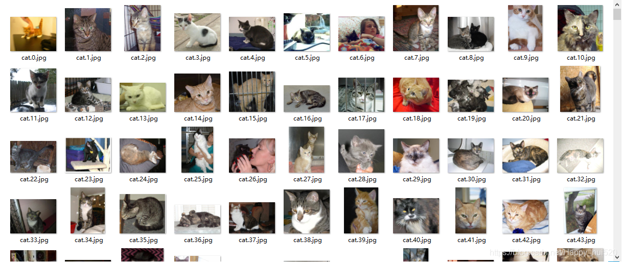
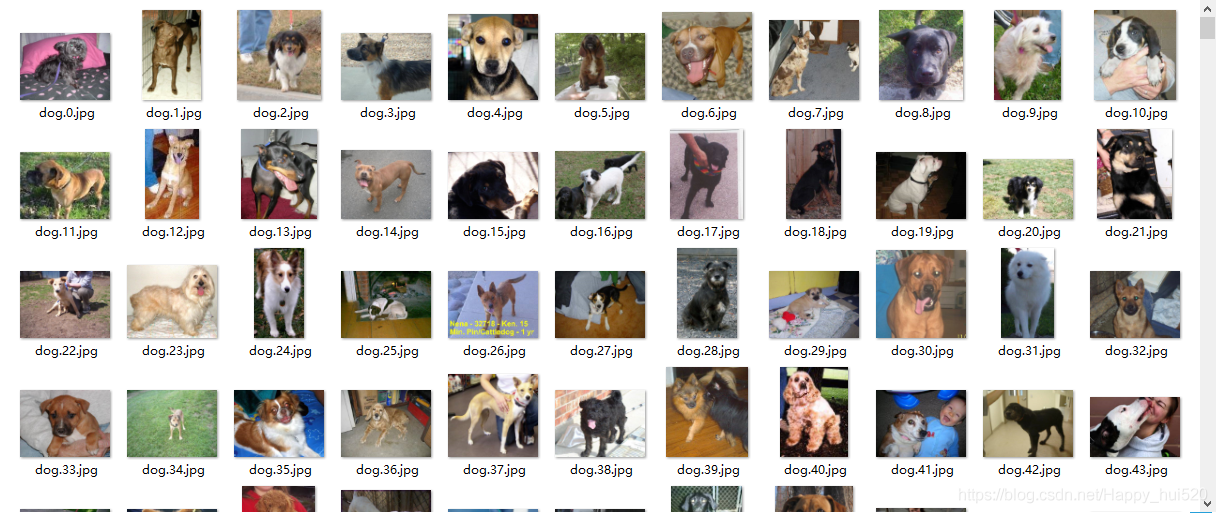
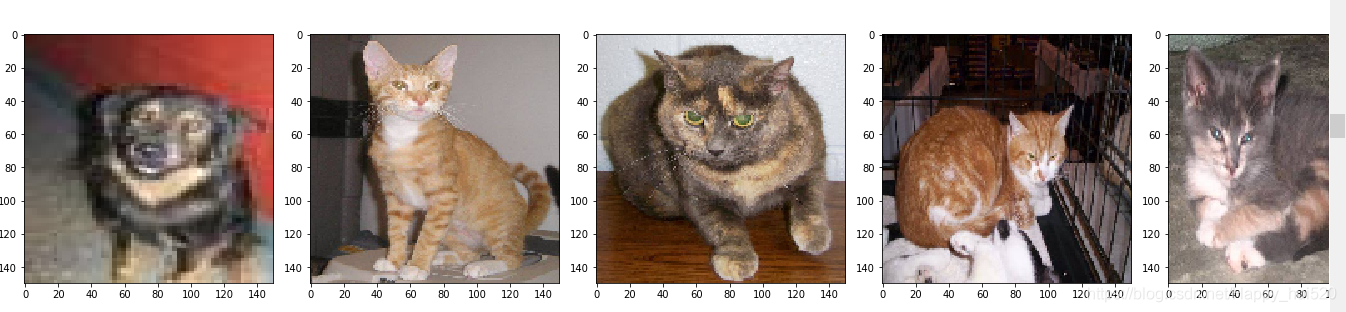
部分数据集：

还有一只小可爱~

项目准备

需要懂CNN（卷积神经网络）的基础知识，知道数据在CNN中是如何传递的，有Python语法基础。

提前下载好dogs-vs-cats 数据集（https://storage.googleapis.com/mledu-datasets/cats_and_dogs_filtered.zip）。

需要安装好pillow、scipy模块，代码中相关模块会用到。

项目代码

Importing packages

# Importing packages
# 这句话是针对python2.x版本做的兼容处理，使2.x版本按新版本的规则进行导入、除法、打印、Unicode文本处理
from __future__ import absolute_import, division, print_function, unicode_literals

import os #这个从磁盘读取文件信息时要用
import matplotlib.pyplot as plt
import numpy as np

import tensorflow as tf
from tensorflow.keras.preprocessing.image import ImageDataGenerator

import logging
logger = tf.get_logger()
logger.setLevel(logging.ERROR) # 使TensorFlow只提示ERROR

Data Loading

注意要把你已经解压的数据集的存储位置赋值给base_dir变量

"""
# 谷歌的链接，国内不能直接访问，可以先下载下来手动配置。
_URL = 'https://storage.googleapis.com/mledu-datasets/cats_and_dogs_filtered.zip'
# 返回文件存储目录(含文件名)
zip_dir = tf.keras.utils.get_file('cats_and_dogs_filterted.zip', origin=_URL, extract=True)
# os.path.dirname() 去掉文件名，返回目录
base_dir = os.path.join(os.path.dirname(zip_dir), 'cats_and_dogs_filtered')
"""

# 这里直接设置数据集路径（已经下载并解压）
base_dir = r'C:\Users\DELL\.keras\datasets\cats_and_dogs_filtered'
train_dir = os.path.join(base_dir, 'train')
validation_dir = os.path.join(base_dir, 'validation')

train_cats_dir = os.path.join(train_dir, 'cats')  # directory with our training cat pictures
train_dogs_dir = os.path.join(train_dir, 'dogs')  # directory with our training dog pictures
validation_cats_dir = os.path.join(validation_dir, 'cats')  # directory with our validation cat pictures
validation_dogs_dir = os.path.join(validation_dir, 'dogs')  # directory with our validation dog pictures

我试了一下发现有时候也能从程序里下载数据集，只不过速度很慢（最后快下载完了不动了，失败了）。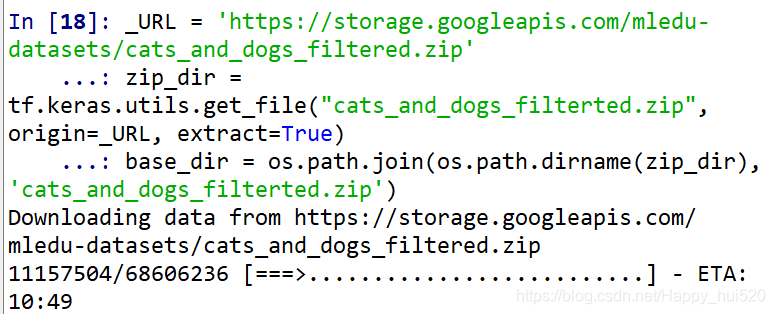

Understanding our data

num_cats_tr = len(os.listdir(train_cats_dir))
num_dogs_tr = len(os.listdir(train_dogs_dir))

num_cats_val = len(os.listdir(validation_cats_dir))
num_dogs_val = len(os.listdir(validation_dogs_dir))

total_train = num_cats_tr + num_dogs_tr
total_val = num_cats_val + num_dogs_val

print('total training cat images:', num_cats_tr)
print('total training dog images:', num_dogs_tr)

print('total validation cat images:', num_cats_val)
print('total validation dog images:', num_dogs_val)
print("--")
print("Total training images:", total_train)
print("Total validation images:", total_val)

Setting Model Parameters

# Setting Model Parameters
BATCH_SIZE = 100  # Number of training examples to process before updating our models variables
IMG_SHAPE  = 150  # Our training data consists of images with width of 150 pixels and height of 150 pixels

Data Preparation

# Data Preparation
train_image_generator      = ImageDataGenerator(rescale=1./255)  # Generator for our training data
validation_image_generator = ImageDataGenerator(rescale=1./255)  # Generator for our validation data

train_data_gen = train_image_generator.flow_from_directory(batch_size=BATCH_SIZE, 
                                                           directory=train_dir, 
                                                           shuffle=True, 
                                                           target_size=(IMG_SHAPE,IMG_SHAPE), #(150,150) 
                                                           class_mode='binary')

val_data_gen = validation_image_generator.flow_from_directory(batch_size=BATCH_SIZE, 
                                                              directory=validation_dir,
                                                              shuffle=False,
                                                              target_size=(IMG_SHAPE,IMG_SHAPE), #(150,150)
                                                              class_mode='binary')

Visualizing Training images

 # Visualizing Training images
sample_training_images, _ = next(train_data_gen) 

# This function will plot images in the form of a grid with 1 row and 5 columns where images are placed in each column.
def plotImages(images_arr):
    fig, axes = plt.subplots(1, 5, figsize=(20,20))
    axes = axes.flatten()
    for img, ax in zip( images_arr, axes):
        ax.imshow(img)
    plt.tight_layout()
    plt.show()
    
plotImages(sample_training_images[:5])  # Plot images 0-4

把图像收缩成150*150之后模糊了很多，看着有点凶呀~

Model Creation

Define the model

model = tf.keras.models.Sequential([
    tf.keras.layers.Conv2D(32, (3,3), activation='relu', input_shape=(150, 150, 3)),
    tf.keras.layers.MaxPooling2D(2, 2),

    tf.keras.layers.Conv2D(64, (3,3), activation='relu'),
    tf.keras.layers.MaxPooling2D(2,2),
    
    tf.keras.layers.Conv2D(128, (3,3), activation='relu'),
    tf.keras.layers.MaxPooling2D(2,2),
    
    tf.keras.layers.Conv2D(128, (3,3), activation='relu'),
    tf.keras.layers.MaxPooling2D(2,2),
    
    tf.keras.layers.Flatten(),
    tf.keras.layers.Dense(512, activation='relu'),
    tf.keras.layers.Dense(2, activation='softmax')
])

注意，最后一个层级（分类器）由一个 Dense 层（具有 2 个输出单元）和一个 softmax 激活函数组成，如下所示：
     tf.keras.layers.Dense(2, activation='softmax')
在处理二元分类问题时，另一个常见方法是：分类器由一个 Dense 层（具有 1 个输出单元）和一个 sigmoid 激活函数组成，如下所示：
     tf.keras.layers.Dense(1, activation='sigmoid')
这两种方法都适合二元分类问题，但是请注意，如果决定在分类器中使用 sigmoid 激活函数，需要将 model.compile() 方法中的 loss 参数从 'sparse_categorical_crossentropy' 更改为'binary_crossentropy'，如下所示：
model.compile(optimizer='adam', 
              loss='binary_crossentropy',
              metrics=['accuracy'])

Compile the model

model.compile(optimizer='adam', 
              loss='sparse_categorical_crossentropy',
              metrics=['accuracy'])

Model Summary

查看刚才建好的模型的信息（其实可以用tensorboard进行可视化显示的，这个我还不会emmmm）

model.summary()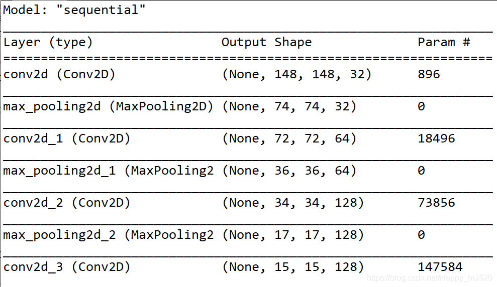

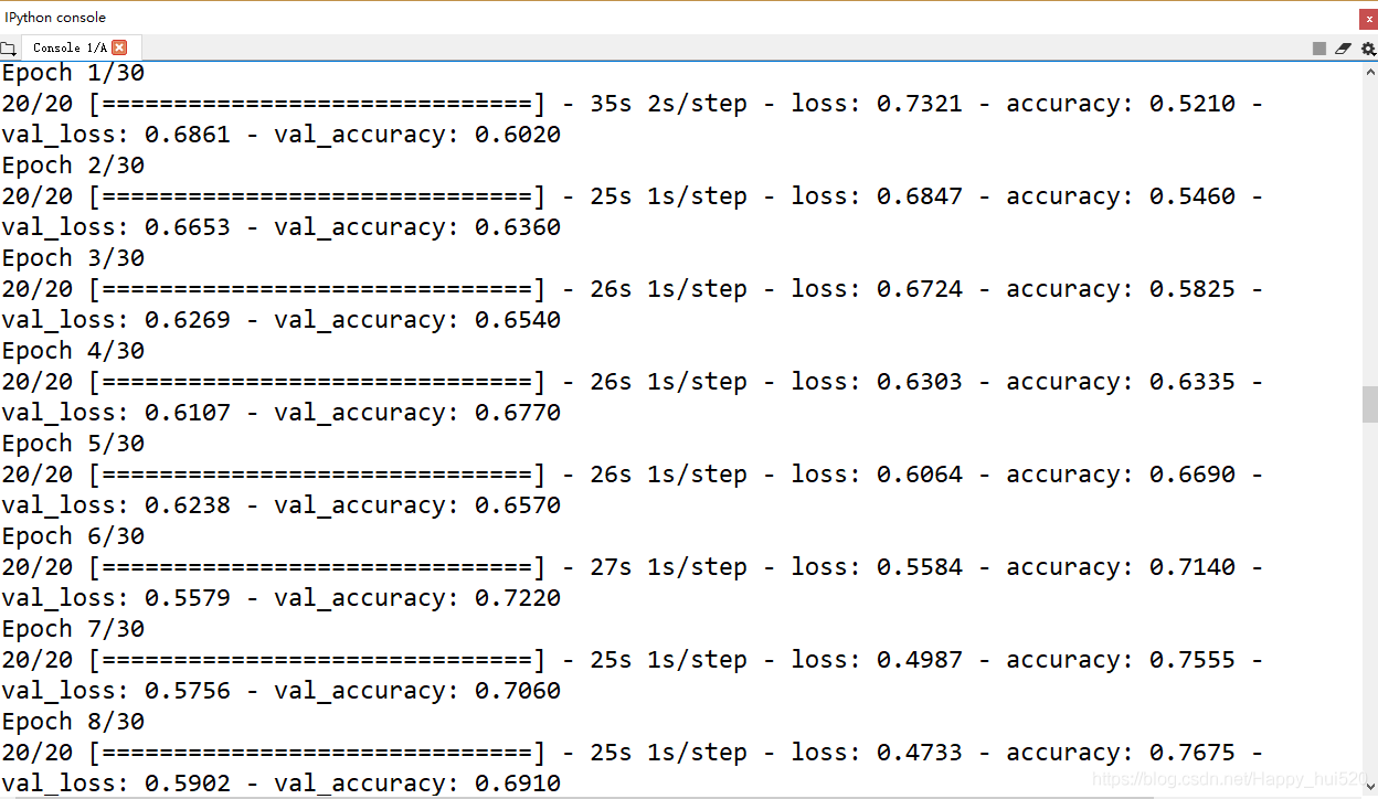
Train the model

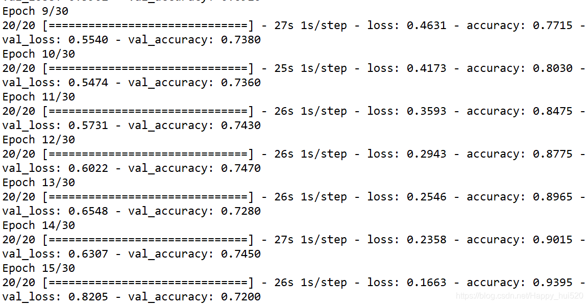
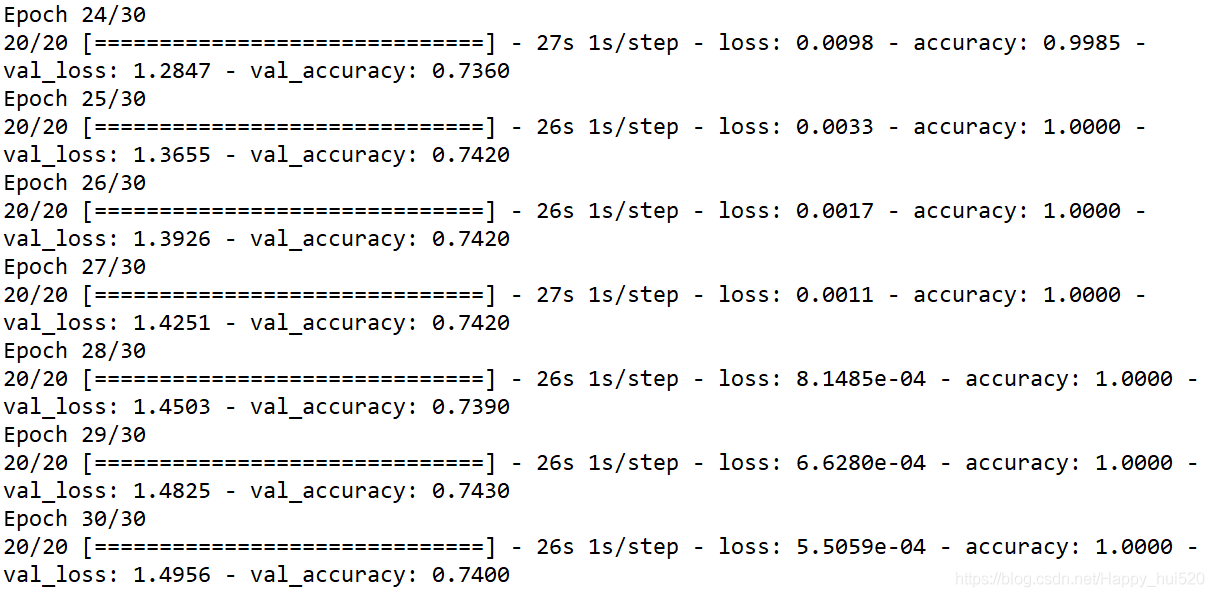
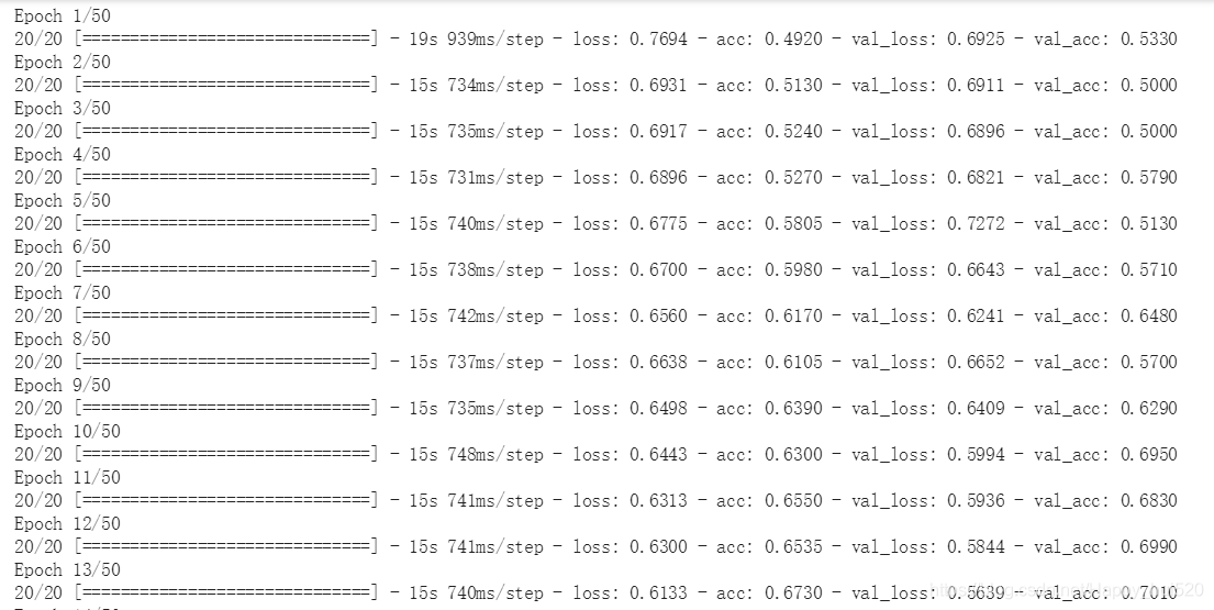
这里的epochs可以自己改改试试，CNN提取特征能力很强大，10个迭代期左右就已经过拟合了。然后你会看到训练集的accuracy不断上升直到1（100%），测试集的accuracy却只有0.7多一点，有时候还在下降。

EPOCHS = 30
history = model.fit_generator(
    train_data_gen,
    steps_per_epoch=int(np.ceil(total_train / float(BATCH_SIZE))),
    epochs=EPOCHS,
    validation_data=val_data_gen,
    validation_steps=int(np.ceil(total_val / float(BATCH_SIZE)))
)

Visualizing results of the training

这一步是打印训练过程中训练集和测试集的accuracy、Loss曲线，看一下过拟合的情况。

# Visualizing results of the training
acc = history.history['accuracy']
val_acc = history.history['val_accuracy']

loss = history.history['loss']
val_loss = history.history['val_loss']

epochs_range = range(EPOCHS)

plt.figure(figsize=(8, 8))
plt.subplot(1, 2, 1)
plt.plot(epochs_range, acc, label='Training Accuracy')
plt.plot(epochs_range, val_acc, label='Validation Accuracy')
plt.legend(loc='lower right')
plt.title('Training and Validation Accuracy')

plt.subplot(1, 2, 2)
plt.plot(epochs_range, loss, label='Training Loss')
plt.plot(epochs_range, val_loss, label='Validation Loss')
plt.legend(loc='upper right')
plt.title('Training and Validation Loss')
plt.savefig('./foo.png')
plt.show()

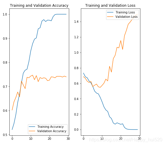
可以很明显的看到，第8个迭代期之后就开始过拟合了，测试集的Loss不降反升，训练集的Loss最终下降到0。

解决过拟合问题

主要采取三种解决方式：

Data Augmentation(数据增强)

通过向训练集中的现有图像应用随机图像转换，人为地增加训练集中的图像数量。

Overfitting often occurs when we have a small number of training examples. One way to fix this problem is to augment our dataset so that it has sufficient number and variety of training examples. Data augmentation takes the approach of generating more training data from existing training samples, by augmenting the samples through random transformations that yield believable-looking images. The goal is that at training time, your model will never see the exact same picture twice. This exposes the model to more aspects of the data, allowing it to generalize better.

In tf.keras we can implement this using the same ImageDataGenerator class we used before. We can simply pass different transformations we would want to our dataset as a form of arguments and it will take care of applying it to the dataset during our training process.

To start off, let's define a function that can display an image, so we can see the type of augmentation that has been performed. Then, we'll look at specific augmentations that we'll use during training.

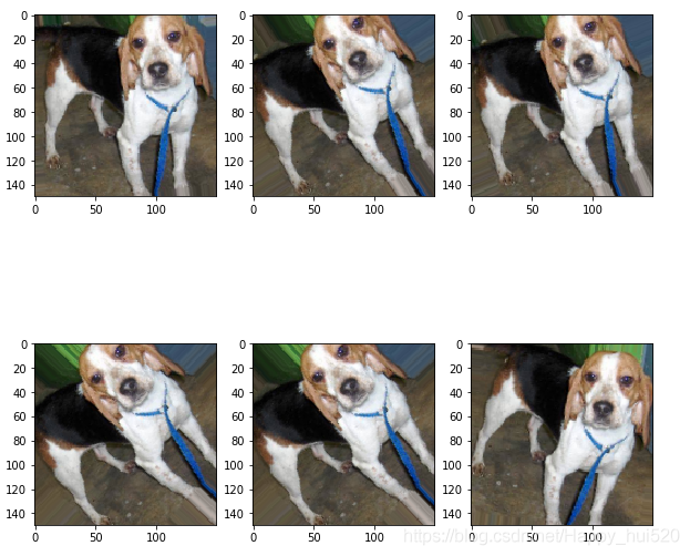
Flipping the image horizontally

image_gen = ImageDataGenerator(rescale=1./255, horizontal_flip=True)

# train_data_gen是一个目录迭代器（Directory Iterator）
train_data_gen = image_gen.flow_from_directory(batch_size=BATCH_SIZE, 
                                               directory=train_dir, 
                                               shuffle=True, 
                                               target_size=(IMG_SHAPE,IMG_SHAPE)
                                              )
augmented_images = [train_data_gen[0][0][1] for i in range(6)] #从生成器里“取数据”，每次都随机应用指定的变换
plotImages(augmented_images)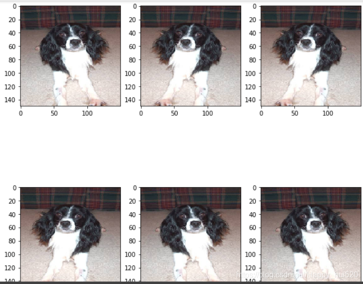

Rotating the image

image_gen = ImageDataGenerator(rescale=1./255, rotation_range=60)

train_data_gen = image_gen.flow_from_directory(batch_size=BATCH_SIZE, 
                                               directory=train_dir, 
                                               shuffle=True, 
                                               target_size=(IMG_SHAPE, IMG_SHAPE))
augmented_images = [train_data_gen[0][0][0] for i in range(6)]
plotImages(augmented_images)

Applying Zoom

image_gen = ImageDataGenerator(rescale=1./255,   
      zoom_range=0.5)

train_data_gen = image_gen.flow_from_directory(batch_size=BATCH_SIZE, 
                                               directory=train_dir, 
                                               shuffle=True, 
                                               target_size=(IMG_SHAPE, IMG_SHAPE))

augmented_images = [train_data_gen[0][0][2] for i in range(6)]
plotImages(augmented_images)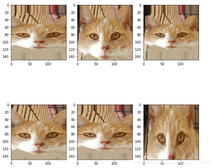

Putting it all together

We can apply all these augmentations, and even others, with just one line of code, by passing the augmentations as arguments with proper values.

Here, we have applied rescale, rotation of 45 degrees, width shift, height shift, horizontal flip, and zoom augmentation to our training images.

image_gen_train = ImageDataGenerator(
      rescale=1./255,
      rotation_range=40, 
      width_shift_range=0.2,
      height_shift_range=0.2,
      shear_range=0.2,
      zoom_range=0.2,
      horizontal_flip=True,
      fill_mode='nearest')

train_data_gen = image_gen_train.flow_from_directory(batch_size=BATCH_SIZE, 
                                                     directory=train_dir, 
                                                     shuffle=True, 
                                                     target_size=(IMG_SHAPE,IMG_SHAPE),
                                                     class_mode='binary')
augmented_images = [train_data_gen[0][0][0] for i in range(6)]
plotImages(augmented_images)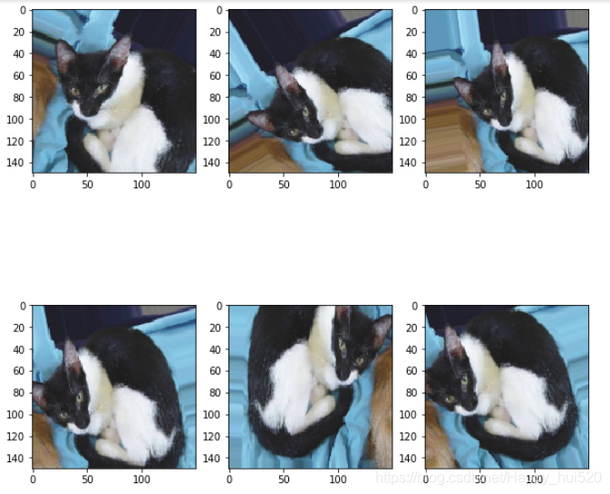

想详细了解 ImageDataGenerator中各个参数的作用可以看这篇博客 https://blog.csdn.net/jacke121/article/details/79245732

Dropout(丢弃法)

在训练过程中，从神经网络中随机选择固定数量的神经元并关闭这些神经元。

这一步应用在创建模型的时候，就是定义一个额外的网络层，设置随机“丢弃”的范围。

model = tf.keras.models.Sequential([
    tf.keras.layers.Conv2D(32, (3,3), activation='relu', input_shape=(150, 150, 3)),
    tf.keras.layers.MaxPooling2D(2, 2),

    tf.keras.layers.Conv2D(64, (3,3), activation='relu'),
    tf.keras.layers.MaxPooling2D(2,2),

    tf.keras.layers.Conv2D(128, (3,3), activation='relu'),
    tf.keras.layers.MaxPooling2D(2,2),

    tf.keras.layers.Conv2D(128, (3,3), activation='relu'),
    tf.keras.layers.MaxPooling2D(2,2),

    tf.keras.layers.Dropout(0.5), #在卷积层后面加一个dropout层
    tf.keras.layers.Flatten(),
    tf.keras.layers.Dense(512, activation='relu'),
    tf.keras.layers.Dense(2, activation='softmax')    
])

Early Stop(早停法)

对于此方法，我们会在训练过程中跟踪验证集的损失，并根据该损失判断何时停止训练，使模型很准确，但是不会过拟合。可以根据实际情况使用，设置损失的范围和容忍的迭代期（epochs），让模型自己停止训练。

但是，这些并非防止过拟合的唯一技巧。请点击以下链接，深入了解这些技巧和其他技巧：

Memorizing is not learning! — 6 tricks to prevent overfitting in machine learning

模型训练

和上面一样，这里直接贴训练结果了。考虑到时间问题，我第一次只训练了50个迭代期，根据accuracy和loss的变化情况来看，神经网络的性能在持续提高。

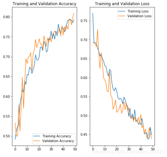
你可能会对上图中大部分情况下验证集的accuracy超过训练集的accuracy感到奇怪，这个其实是容易理解的。经过各种数据增强 的训练集其实更难识别了，而我们没有对验证集作变换，所以它对神经网络更“仁慈”一些。

继续训练看一下什么情况

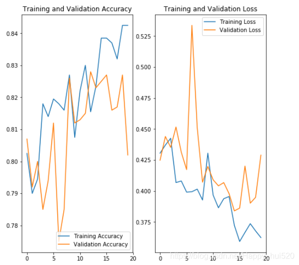
验证集的accuracy差不多最高达到83%，但是可以看出来上升幅度较小了。

这个成绩相比进行过拟合处理之前的结果好了很多，但是错误率仍然较大，达不到我们的期望。

迁移学习

下一篇博客中，我们将使用迁移学习来提升模型准确度到接近99%！

一念逍遥、

关注

2
点赞
踩
9

收藏

觉得还不错? 一键收藏
0
评论
TensorFlow + Keras 图像识别：Dogs vs Cats Image Classification with data augmentation(CNN, 解决过拟合问题)

OS：Win10Interpreter: Python3.7Environment: Anaconda3 + Tensorflow-gpu2.0.0 + SpyderAPI: tf.keras(a high-level API to build and train models in TensorFlow)项目源码参考自TensorFlow官方教程https://colab.r...
复制链接

扫一扫