


基于SegNet的无人驾驶场景理解研究与实现
一、研究背景
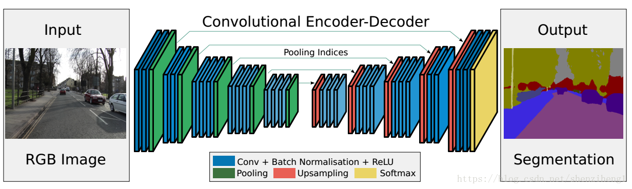
SegNet是一种基于卷积神经网络的图像分割技术,广泛用于场景理解领域。在无人驾驶技术中,需要对道路场景进行实时分割以提取车辆、路面、道路标识等关键信息,进而支持车辆决策和控制。
SegNet通过对图像进行特征提取、编码、解码等操作,来识别图像中不同的场景元素。在实现过程中,需要选择合适的数据集、设计合理的网络结构,并通过不断的训练和评估来提高模型的分割准确度。
具体来说,就是对一张道路图片,逐像素分析为每一个像素点分配语义标签,并用不同颜色标出;最终对图片中的各个类别物体涂上不同的颜色。
二、实现步骤
基于SegNet的无人驾驶场景理解研究与实现包括以下几个步骤:
- 数据集选择:选择包含道路场景的图像数据集,用于训练和评估模型。
- 网络结构设计:设计符合场景分割任务要求的SegNet网络结构,比如使用不同的卷积层等。
- 损失函数:设计合适的损失函数来更新网络中的参数。
- 训练和评估:使用训练数据集训练SegNet模型,不断迭代以提高模型的分割准确度,并使用测试数据集评估模型的分割结果。
数据集的选择
使用了cityscapes-dataset中公开的数据集,数据集包括:3475张用于训练和验证的图片及对应分割好的结果图片、1525张用于测试的图片及对应分割好的结果图片;
数据集的下载:


网络结构设计
经典的SegNet网络结构:
输入——2层卷积——1层池化 2层卷积——1层池化
3层卷积——1层池化 3层卷积——1层池化
3层卷积——1层池化 1层上采样——3层卷积
1层上采样——3层卷积 1层上采样——3层卷积
1层上采样——2层卷积 1层上采样——2层卷积——输出
==========================================================================================
Layer (type:depth-idx)                   Output Shape              Param #
==========================================================================================
SegNet                                     ——         			    --
├─single_conv: 1-1                       [1, 64, 96, 96]           --
│    └─Conv2d: 2-1                       [1, 64, 96, 96]           1,792
│    └─BatchNorm2d: 2-2                  [1, 64, 96, 96]           128
│    └─ReLU: 2-3                         [1, 64, 96, 96]           --
├─single_conv: 1-2                       [1, 64, 96, 96]           --
│    └─Conv2d: 2-4                       [1, 64, 96, 96]           36,928
│    └─BatchNorm2d: 2-5                  [1, 64, 96, 96]           128
│    └─ReLU: 2-6                         [1, 64, 96, 96]           --
├─down_layer: 1-3                        [1, 64, 48, 48]           --
│    └─MaxPool2d: 2-7                    [1, 64, 48, 48]           --
├─single_conv: 1-4                       [1, 128, 48, 48]          --
│    └─Conv2d: 2-8                       [1, 128, 48, 48]          73,856
│    └─BatchNorm2d: 2-9                  [1, 128, 48, 48]          256
│    └─ReLU: 2-10                        [1, 128, 48, 48]          --
├─single_conv: 1-5                       [1, 128, 48, 48]          --
│    └─Conv2d: 2-11                      [1, 128, 48, 48]          147,584
│    └─BatchNorm2d: 2-12                 [1, 128, 48, 48]          256
│    └─ReLU: 2-13                        [1, 128, 48, 48]          --
├─down_layer: 1-6                        [1, 128, 24, 24]          --
│    └─MaxPool2d: 2-14                   [1, 128, 24, 24]          --
├─single_conv: 1-7                       [1, 256, 24, 24]          --
│    └─Conv2d: 2-15                      [1, 256, 24, 24]          295,168
│    └─BatchNorm2d: 2-16                 [1, 256, 24, 24]          512
│    └─ReLU: 2-17                        [1, 256, 24, 24]          --
├─single_conv: 1-8                       [1, 256, 24, 24]          --
│    └─Conv2d: 2-18                      [1, 256, 24, 24]          590,080
│    └─BatchNorm2d: 2-19                 [1, 256, 24, 24]          512
│    └─ReLU: 2-20                        [1, 256, 24, 24]          --
├─single_conv: 1-9                       [1, 256, 24, 24]          --
│    └─Conv2d: 2-21                      [1, 256, 24, 24]          590,080
│    └─BatchNorm2d: 2-22                 [1, 256, 24, 24]          512
│    └─ReLU: 2-23                        [1, 256, 24, 24]          --
├─down_layer: 1-10                       [1, 256, 12, 12]          --
│    └─MaxPool2d: 2-24                   [1, 256, 12, 12]          --
├─single_conv: 1-11                      [1, 512, 12, 12]          --
│    └─Conv2d: 2-25                      [1, 512, 12, 12]          1,180,160
│    └─BatchNorm2d: 2-26                 [1, 512, 12, 12]          1,024
│    └─ReLU: 2-27                        [1, 512, 12, 12]          --
├─single_conv: 1-12                      [1, 512, 12, 12]          --
│    └─Conv2d: 2-28                      [1, 512, 12, 12]          2,359,808
│    └─BatchNorm2d: 2-29                 [1, 512, 12, 12]          1,024
│    └─ReLU: 2-30                        [1, 512, 12, 12]          --
├─single_conv: 1-13                      [1, 512, 12, 12]          --
│    └─Conv2d: 2-31                      [1, 512, 12, 12]          2,359,808
│    └─BatchNorm2d: 2-32                 [1, 512, 12, 12]          1,024
│    └─ReLU: 2-33                        [1, 512, 12, 12]          --
├─down_layer: 1-14                       [1, 512, 6, 6]            --
│    └─MaxPool2d: 2-34                   [1, 512, 6, 6]            --
├─single_conv: 1-15                      [1, 512, 6, 6]            --
│    └─Conv2d: 2-35                      [1, 512, 6, 6]            2,359,808
│    └─BatchNorm2d: 2-36                 [1, 512, 6, 6]            1,024
│    └─ReLU: 2-37                        [1, 512, 6, 6]            --
├─single_conv: 1-16                      [1, 512, 6, 6]            --
│    └─Conv2d: 2-38                      [1, 512, 6, 6]            2,359,808
│    └─BatchNorm2d: 2-39                 [1, 512, 6, 6]            1,024
│    └─ReLU: 2-40                        [1, 512, 6, 6]            --
├─single_conv: 1-17                      [1, 512, 6, 6]            --
│    └─Conv2d: 2-41                      [1, 512, 6, 6]            2,359,808
│    └─BatchNorm2d: 2-42                 [1, 512, 6, 6]            1,024
│    └─ReLU: 2-43                        [1, 512, 6, 6]            --
├─down_layer: 1-18                       [1, 512, 3, 3]            --
│    └─MaxPool2d: 2-44                   [1, 512, 3, 3]            --
├─un_pool: 1-19                          [1, 512, 6, 6]            --
│    └─MaxUnpool2d: 2-45                 [1, 512, 6, 6]            --
├─single_conv: 1-20                      [1, 512, 6, 6]            --
│    └─Conv2d: 2-46                      [1, 512, 6, 6]            2,359,808
│    └─BatchNorm2d: 2-47                 [1, 512, 6, 6]            1,024
│    └─ReLU: 2-48                        [1, 512, 6, 6]            --
├─single_conv: 1-21                      [1, 512, 6, 6]            --
│    └─Conv2d: 2-49                      [1, 512, 6, 6]            2,359,808
│    └─BatchNorm2d: 2-50                 [1, 512, 6, 6]            1,024
│    └─ReLU: 2-51                        [1, 512, 6, 6]            --
├─single_conv: 1-22                      [1, 512, 6, 6]            --
│    └─Conv2d: 2-52                      [1, 512, 6, 6]            2,359,808
│    └─BatchNorm2d: 2-53                 [1, 512, 6, 6]            1,024
│    └─ReLU: 2-54                        [1, 512, 6, 6]            --
├─un_pool: 1-23                          [1, 512, 12, 12]          --
│    └─MaxUnpool2d: 2-55                 [1, 512, 12, 12]          --
├─single_conv: 1-24                      [1, 512, 12, 12]          --
│    └─Conv2d: 2-56                      [1, 512, 12, 12]          2,359,808
│    └─BatchNorm2d: 2-57                 [1, 512, 12, 12]          1,024
│    └─ReLU: 2-58                        [1, 512, 12, 12]          --
├─single_conv: 1-25                      [1, 512, 12, 12]          --
│    └─Conv2d: 2-59                      [1, 512, 12, 12]          2,359,808
│    └─BatchNorm2d: 2-60                 [1, 512, 12, 12]          1,024
│    └─ReLU: 2-61                        [1, 512, 12, 12]          --
├─single_conv: 1-26                      [1, 256, 12, 12]          --
│    └─Conv2d: 2-62                      [1, 256, 12, 12]          1,179,904
│    └─BatchNorm2d: 2-63                 [1, 256, 12, 12]          512
│    └─ReLU: 2-64                        [1, 256, 12, 12]          --
├─un_pool: 1-27                          [1, 256, 24, 24]          --
│    └─MaxUnpool2d: 2-65                 [1, 256, 24, 24]          --
├─single_conv: 1-28                      [1, 256, 24, 24]          --
│    └─Conv2d: 2-66                      [1, 256, 24, 24]          590,080
│    └─BatchNorm2d: 2-67                 [1, 256, 24, 24]          512
│    └─ReLU: 2-68                        [1, 256, 24, 24]          --
├─single_conv: 1-29                      [1, 256, 24, 24]          --
│    └─Conv2d: 2-69                      [1, 256, 24, 24]          590,080
│    └─BatchNorm2d: 2-70                 [1, 256, 24, 24]          512
│    └─ReLU: 2-71                        [1, 256, 24, 24]          --
├─single_conv: 1-30                      [1, 128, 24, 24]          --
│    └─Conv2d: 2-72                      [1, 128, 24, 24]          295,040
│    └─BatchNorm2d: 2-73                 [1, 128, 24, 24]          256
│    └─ReLU: 2-74                        [1, 128, 24, 24]          --
├─un_pool: 1-31                          [1, 128, 48, 48]          --
│    └─MaxUnpool2d: 2-75                 [1, 128, 48, 48]          --
├─single_conv: 1-32                      [1, 128, 48, 48]          --
│    └─Conv2d: 2-76                      [1, 128, 48, 48]          147,584
│    └─BatchNorm2d: 2-77                 [1, 128, 48, 48]          256
│    └─ReLU: 2-78                        [1, 128, 48, 48]          --
├─single_conv: 1-33                      [1, 64, 48, 48]           --
│    └─Conv2d: 2-79                      [1, 64, 48, 48]           73,792
│    └─BatchNorm2d: 2-80                 [1, 64, 48, 48]           128
│    └─ReLU: 2-81                        [1, 64, 48, 48]           --
├─un_pool: 1-34                          [1, 64, 96, 96]           --
│    └─MaxUnpool2d: 2-82                 [1, 64, 96, 96]           --
├─single_conv: 1-35                      [1, 64, 96, 96]           --
│    └─Conv2d: 2-83                      [1, 64, 96, 96]           36,928
│    └─BatchNorm2d: 2-84                 [1, 64, 96, 96]           128
│    └─ReLU: 2-85                        [1, 64, 96, 96]           --
├─outconv: 1-36                          [1, 20, 96, 96]           --
│    └─Conv2d: 2-86                      [1, 20, 96, 96]           11,540
==========================================================================================
Total params: 29,454,548
Trainable params: 29,454,548
Non-trainable params: 0
Total mult-adds (G): 5.73
==========================================================================================
Input size (MB): 0.11
Forward/backward pass size (MB): 67.53
Params size (MB): 117.82
Estimated Total Size (MB): 185.46
==========================================================================================
损失函数
在不同的应用场景中,不同的物体具有不同的重要性和安全相关性,传统的损失函数,如交叉熵,并没有考虑到不同交通元素的不同重要性,例如:汽车和行人在自动驾驶中最为重要,所以在场景分割时,场景分割的结果应该更倾向于重要的类。参考资料,我们找到了一个重要性感知的损失函数,可以根据现实世界的应用分配语义的重要性。
论文中例子:
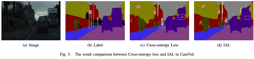
可以看出方框中采用常规的交叉熵函数会被预测为树木的部分,在采用IAL后被倾向于预测为公交车,这与实际情况是符合的。
IAL在避免把重要的类预测成不重要的类的错误的情况,即使可能有部分不重要的类被预测为重要的类。用该重要性感知的损失函数更新参数,在实际自动驾驶中可以避免严重的事故的发生。
训练和评估
训练100轮,取验证集上损失函数的值最小的模型保存下来,并根据该模型在测试集上进行评估和可视化结果。
三、代码实现及详解
实现环境:Google colab Pro
准备工作(库和模块的导入)
可视化进度条
# 安装可以可视化进度条的库pytorch-ignite
!pip install pytorch-ignite
使用这个库训练模型时,不需要写一大堆前向传播,后向传播等代码,直接调用库,就可以可视化loss、准确率、训练轮数的进度条;
导入使用的模块
import os
import cv2
import glob
import torch
import numpy as np
import pandas as pd
import seaborn as sns
import matplotlib.pyplot as plt
from tqdm import tqdm

from ignite.metrics.confusion_matrix import ConfusionMatrix
from ignite.metrics import mIoU, IoU

import torchvision.transforms as transforms
import torchvision.datasets as datasets

import torch.nn as nn
import torch.nn.functional as F
import torchvision
import random
from random import randint
from torch import optim

np.set_printoptions(precision=3, suppress=True)
# 控制输出结果的精度为3(即小数点后为3位),且小数以科学记数法表示;
数据集导入及数据的处理
数据集导入
如果在本地运行,直接将数据集和代码放在同级目录下;如果在google的colab上运行,需要先将数据集上传到google云盘,之后访问google云盘,将路径切换到云盘下;
# 安装google驱动器以访问数据集(在本机上运行时将以下代码注释)
from google.colab import drive
import os
# 挂载网盘
drive.mount('/content/drive/')
# 切换路径
os.chdir('/content/drive/MyDrive/ColabNotebooks/SegNetonCityscapes-main')
Google的colab中,可以直接在代码行中输入!ls查看当前所在的文件目录,执行完上述代码之后当前文件路径应该变为:Mounted at /content/drive。
!ls
demo.pth		  net.pt     SegNetandIAL.ipynb		 url.txt
gtFine_trainvaltest	  README.md  SegNet_on_cityscapes.ipynb  visdomlog.txt
leftImg8bit_trainvaltest  runs	     SegNet场景分割.ipynb
# 定义训练和验证数据集的文件路径
train_label_data_path  = './gtFine_trainvaltest/gtFine/train'
valid_label_data_path  = './gtFine_trainvaltest/gtFine/val'
train_img_path  = './leftImg8bit_trainvaltest/leftImg8bit/train'
valid_img_path  = './leftImg8bit_trainvaltest/leftImg8bit/val'
# 匹配各类图像文件的文件路径,保存在各个列表中,并对各列表进行排序
train_labels = sorted(glob.glob(train_label_data_path+"/*/*_labelIds.png"))
valid_labels = sorted(glob.glob(valid_label_data_path+"/*/*_labelIds.png"))
train_inp = sorted(glob.glob(train_img_path+"/*/*.png"))
valid_inp = sorted(glob.glob(valid_img_path+"/*/*.png"))
此时train_labels列表内的部分如下:
['./gtFine_trainvaltest/gtFine/train/aachen/aachen_000000_000019_gtFine_labelIds.png',
 './gtFine_trainvaltest/gtFine/train/aachen/aachen_000001_000019_gtFine_labelIds.png',
 './gtFine_trainvaltest/gtFine/train/aachen/aachen_000002_000019_gtFine_labelIds.png',
 './gtFine_trainvaltest/gtFine/train/aachen/aachen_000003_000019_gtFine_labelIds.png',
 './gtFine_trainvaltest/gtFine/train/aachen/aachen_000004_000019_gtFine_labelIds.png',
 './gtFine_trainvaltest/gtFine/train/aachen/aachen_000005_000019_gtFine_labelIds.png',
 './gtFine_trainvaltest/gtFine/train/aachen/aachen_000006_000019_gtFine_labelIds.png',
 './gtFine_trainvaltest/gtFine/train/aachen/aachen_000007_000019_gtFine_labelIds.png',
 './gtFine_trainvaltest/gtFine/train/aachen/aachen_000008_000019_gtFine_labelIds.png',
 ...]
此时满足训练集(train_labels)中第一张图片对应的分割,恰好是训练集分割(train_inp)中的第一张图片,以此类推,训练集和训练集的分割、验证集和验证集的分割,都是一一有序对应的。
Label和Label有关的元数据信息
from collections import namedtuple

Label = namedtuple( 'Label' , [
    'name'        , # label的名字,例如:car、person...,注意名字不会重复
    'id'          , # 一个label唯一对应一个不重复的Id
    'trainId'     , # 对用于训练的label设置的Id,由用户自己制定,可以重复
    'ignoreInEval', # 在评估过程中,是否忽略该label
    'color'       , # label对应的颜色
    ] )
namedtuple介绍
Python 中的 namedtuple 是一种不可变的、命名的元组。与普通元组不同,namedtuple 元素可以通过名称访问,而不仅仅是通过索引。
collections.namedtuple(typename, field_names, *, verbose=False, rename=False, module=None)
命名元组的语法更加清晰,代码更加简洁,而且易于阅读和维护,因此在一些特定场景下它是非常有用的,例如数据处理和结构化数据存储。
具体的各label的信息
#--------------------------------------------------------------------------------
# 所有标签的信息;
#--------------------------------------------------------------------------------

labels = [
    Label(  'unlabeled'            ,  0 ,      255 ,  True         , (  0,  0,  0) ),
    Label(  'ego vehicle'          ,  1 ,      255 ,  True         , (  0,  0,  0) ),
    Label(  'rectification border' ,  2 ,      255 ,  True         , (  0,  0,  0) ),
    Label(  'out of roi'           ,  3 ,      255 ,  True         , (  0,  0,  0) ),
    Label(  'static'               ,  4 ,      255 ,  True         , (  0,  0,  0) ),
    Label(  'dynamic'              ,  5 ,      255 ,  True         , (111, 74,  0) ),
    Label(  'ground'               ,  6 ,      255 ,  True         , ( 81,  0, 81) ),
    Label(  'road'                 ,  7 ,        0 ,  False        , (128, 64,128) ),
    Label(  'sidewalk'             ,  8 ,        1 ,  False        , (244, 35,232) ),
    Label(  'parking'              ,  9 ,      255 ,  True         , (250,170,160) ),
    Label(  'rail track'           , 10 ,      255 ,  True         , (230,150,140) ),
    Label(  'building'             , 11 ,        2 ,  False        , ( 70, 70, 70) ),
    Label(  'wall'                 , 12 ,        3 ,  False        , (102,102,156) ),
    Label(  'fence'                , 13 ,        4 ,  False        , (190,153,153) ),
    Label(  'guard rail'           , 14 ,      255 ,  True         , (180,165,180) ),
    Label(  'bridge'               , 15 ,      255 ,  True         , (150,100,100) ),
    Label(  'tunnel'               , 16 ,      255 ,  True         , (150,120, 90) ),
    Label(  'pole'                 , 17 ,        5 ,  False        , (153,153,153) ),
    Label(  'polegroup'            , 18 ,      255 ,  True         , (153,153,153) ),
    Label(  'traffic light'        , 19 ,        6 ,  False        , (250,170, 30) ),
    Label(  'traffic sign'         , 20 ,        7 ,  False        , (220,220,  0) ),
    Label(  'vegetation'           , 21 ,        8 ,  False        , (107,142, 35) ),
    Label(  'terrain'              , 22 ,        9 ,  False        , (152,251,152) ),
    Label(  'sky'                  , 23 ,       10 ,  False        , ( 70,130,180) ),
    Label(  'person'               , 24 ,       11 ,  False        , (220, 20, 60) ),
    Label(  'rider'                , 25 ,       12 ,  False        , (255,  0,  0) ),
    Label(  'car'                  , 26 ,       13 ,  False        , (  0,  0,142) ),
    Label(  'truck'                , 27 ,       14 ,  False        , (  0,  0, 70) ),
    Label(  'bus'                  , 28 ,       15 ,  False        , (  0, 60,100) ),
    Label(  'caravan'              , 29 ,      255 ,  True         , (  0,  0, 90) ),
    Label(  'trailer'              , 30 ,      255 ,  True         , (  0,  0,110) ),
    Label(  'train'                , 31 ,       16 ,  False        , (  0, 80,100) ),
    Label(  'motorcycle'           , 32 ,       17 ,  False        , (  0,  0,230) ),
    Label(  'bicycle'              , 33 ,       18 ,  False        , (119, 11, 32) ),
    Label(  'license plate'        , -1 ,       -1 ,  True         , (  0,  0,142) ),
]
数据处理
提取用于训练的label
'''
	ignoreinEval==False代表使用该label
	逐一扫描labels命名元组中的每一个label的信息:
		将使用到的label的全部信息都添加到labels_used[]列表中
		将使用到的label的id都添加到ids[]列表中
'''
labels_used = []
ids = []

for i in range(len(labels)):
  if(labels[i].ignoreInEval == False):
    labels_used.append(labels[i])
    ids.append(labels[i].id)
print("number of labels used = " + format(len(labels_used )))
输出:
number of labels used = 19
# 此输出代表使用了19个类
可视化第一张图片的分割
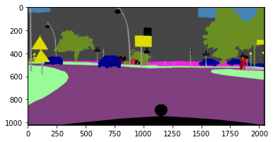
读取
# 读取第一张图片的分割,并且只提取红色通道
label_in = cv2.imread(train_labels[0])[:,:,0]
提取红色通道的原因:标签图片为灰度图,标签信息只在红色通道中保存。
标签图片的例子:

肉眼看上去全黑;
提取红色通道之后:
颜色重覆盖
原来的标签图像为灰度图图像,需要转换为彩色分割图。
同时原来的分割是根据label的id属性来上色的,在训练过程中,我们是根据label的train_id属性进行训练的,故需要将相同train_id但不同id的不同颜色的色块变成相同颜色的色块;实质就是在分割的图像上体现出来由用户自己筛选label用于训练的效果。
例如:原始标签图片中bridge和ground是两类,有两个id,对应两个颜色,但是此时我们将它们的train_Id设置成一样的,训练时就会当成一类,最终bridge和ground就会上色成一个颜色;
创建映射关系
'''
	创建一个以label的id为键、以train_id为值的字典
	id是唯一的,train_id可以重复(重复就是在训练时把它们当成一类,尽管它们本身是不同的物体)
	一个id唯一对应一个train_id
'''

label_dic = {}
for i in range(len(labels)-1):
  label_dic[labels[i].id] = labels[i].trainId
此时label_dic中内容:
{0: 255, 1: 255, 2: 255, 3: 255,
 4: 255, 5: 255, 6: 255, 7: 0,
 8: 1, 9: 255, 10: 255, 11: 2,
 12: 3, 13: 4, 14: 255, 15: 255,
 16: 255, 17: 5, 18: 255, 19: 6,
 20: 7, 21: 8, 22: 9, 23: 10,
 24: 11, 25: 12, 26: 13, 27: 14,
 28: 15, 29: 255, 30: 255, 31: 16,
 32: 17, 33: 18}
train_id为255代表未被筛选出来的类
替换id信息为train_id信息
原始的分割图片中,每一个像素对应一个id,逐像素扫描分割图片,根据label_dic将分割图片中每一个像素的id的信息替换为train_id的信息。
'''
	createtrainID函数:
		将标签图片中用到的label的id信息逐像素换成对应的train_id信息
		输入:
			label_in为原始的分割图像
			label_dic为一个以id为键、以train_id为值的字典
		输出:
			mask矩阵,矩阵大小为图像像素大小,即存有标签图片每个像素点对应的train_id
'''
def createtrainID(label_in,label_dic):
  mask = np.zeros((label_in.shape[0],label_in.shape[1]))
  l_un = np.unique(label_in) # unique()用于去重并排序
  for i in range(len(l_un)):
    mask[label_in==l_un[i]] = label_dic[l_un[i]]
  return mask
重新根据train_id上色
'''
	visual_label()函数:
   	 	根据train_id来重新上色生成训练用的分割图片
   	 	输入:
   	 		mask矩阵:一个图像长*宽大小的矩阵,矩阵中的每一个元素代表图像在该像素点的train_Id;
   	 		labels_used:对图像场景分割时,训练用到的所有label的label信息;
   	 		plot:plot为True时,显示图像;
   	 	输出:
   	 		返回重新上色之后的图片;
'''
def visual_label(mask,labels_used,plot = False):
  label_img = np.zeros((mask.shape[0],mask.shape[1],3))
  # RGB三通道
  r = np.zeros((mask.shape[0],mask.shape[1]))
  g = np.zeros((mask.shape[0],mask.shape[1]))
  b = np.zeros((mask.shape[0],mask.shape[1]))

  l_un = np.unique(mask)
  for i in range(len(l_un)):
    if l_un[i]<19:
      # 分别对三通道上色
      r[mask==int(l_un[i])] = labels_used[int(l_un[i])].color[0]
      g[mask==int(l_un[i])] = labels_used[int(l_un[i])].color[1]
      b[mask==int(l_un[i])] = labels_used[int(l_un[i])].color[2]

  # 将图片像素值归一化到0到1之间的浮点数;
  label_img[:,:,0] = r/255
  label_img[:,:,1] = g/255
  label_img[:,:,2] = b/255

  if plot:
    plt.imshow(label_img)
  return label_img
可视化
label_img = visual_label(createtrainID(label_in,label_dic),labels_used,plot = True)
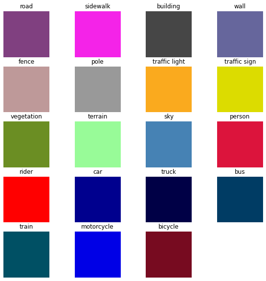
可视化训练使用的label的名称和对应颜色
'''
	不同label采用不同颜色,并可视化类和颜色的对应关系,方便查看上色效果;
'''
fig = plt.figure(figsize = (10,10)) # 创建画布

for i in range(len(labels_used)):
    temp = np.zeros((5,5,3))
    # 分别对三个通道进行颜色归一化;
    temp[:,:,0] = labels_used[i].color[0]/255
    temp[:,:,1] = labels_used[i].color[1]/255
    temp[:,:,2] = labels_used[i].color[2]/255
    # 添加子图
    ax = fig.add_subplot(5, 4, i+1)
    ax.imshow(temp)
    ax.set_title(labels_used[i].name)
    ax.axis('off')
图像处理
对原始图像处理
为了更有效率地进行卷积计算,需要对图像进行缩放处理。图像过大会导致卷积效率降低(存储开销大、卷积计算开销大、卷积核数量多,对卷积核的卷积次数多),因此要将图像缩小到合适的大小,提高卷积效率。
将图像缩放为正方形,可以:
- 提高计算效率:正方形图像可以使用相同大小的卷积核,减少不必要的计算开销。
- 更好的特征提取:正方形图像更容易提取空间特征,因为不会因为长宽比不同而影响卷积结果。
- 简化计算过程:正方形图像不需要进行额外的边缘处理,如填充、裁剪等,因此简化了计算过程。
插值法选择最近邻插值法,直接将新图像中每个像素点映射到原图像中最近的像素点上,插值方式简单,适用于缩放图像且对图像质量要求不高的情况。
'''
	gen_images()函数:
		对用于训练、验证和测试的图像进行处理的函数;
		输入:
			x是读入图像的文件路径的列表,x内有多张图像的文件路径字符串
			s1、s2为调整图像大小后的长和宽
		输出:
			返回图片大小,维度顺序调整之后的图像张量;
'''
def gen_images(x,s1=96,s2=96):
  _,_,s3 = cv2.imread(x[0]).shape # 图片通道数不改变
  img = np.zeros((len(x),s1,s2,s3))
  for i in range(len(x)):
      # 调整图片的大小,resize为s1*s2大小的图片,使用最近邻插值法;
      image= cv2.resize(cv2.imread(x[i]),(s1,s2),interpolation = cv2.INTER_NEAREST)
      image = image/255 # 对每个像素进行归一化处理;
      img[i,:,:,:] = image

  # permute用于调整img维度顺序,使之满足pytorch对维度顺序的要求
  return torch.tensor(img).permute(0,3,1,2)
permute() 函数通常是对图像的维度进行重排的意思。例如,对于一个三维图像,其维度分别为高,宽,通道,如果将其维度重排为通道,高,宽,就可以使用 permute() 函数实现。
重排的目的通常是为了满足深度学习框架的要求,因为不同的深度学习框架对图像的维度要求是不一样的。例如,PyTorch 中要求图像的维度为通道,高,宽,而 Tensorflow 中要求图像的维度为高,宽,通道,因此在使用前需要对图像的维度进行重排。
permute(0,3,1,2)之后图像的维度变为:标识、通道、高、宽,符合PyTorch深度学习的框架对图像维度的要求;
对分割图片处理
'''
	gen_mask_train()函数:
		对用于训练、验证和测试的分割图像进行处理的函数;
		步骤:
			1、将label的id换为train_id
        	2、改变分割图片大小为96*96,与gen_images()之后图片一致
        输入:
        	x是读入图片的文件路径的列表,x内有多张图片的文件路径字符串
        	label_dic为label_id和train_id对应关系的字典类型
        	s1、s2为调整图片大小后的长和宽
        输出:
        	返回图片大小调整后且id换为train_id后的标签图像张量
'''
def gen_mask_train(x,label_dic,s1=96,s2=96):
  mask = np.zeros((len(x),s1,s2))
  for i in range(len(x)):
      # 替换id信息为train_id信息
      image = createtrainID(cv2.resize(cv2.imread(x[i]),(s1,s2),interpolation = cv2.INTER_NEAREST)[:,:,0],label_dic)
      mask[i,:,:] = image
      mask[mask==255] = 19 # 原来255为背景类,将背景类的train_Id设置为19;
  return torch.tensor(mask)
Tensor张量是PyTorch中重要的数据结构,它可以代表一个多维数组,是PyTorch中机器学习和深度学习模型的核心。
Tensor张量具有以下几个特点:
- 可以进行张量运算:如矩阵乘法、张量加法等。
- 可以利用GPU加速:PyTorch的Tensor张量可以自动选择使用GPU加速,从而大幅提高运算效率。
- 可以和autograd模块结合使用:PyTorch的Tensor张量可以和autograd模块结合使用,可以方便地求导、反向传播等。
以张量形式返回可以更好地部署在GPU上。
数据集处理
打乱数据
打乱数据是为了防止出现过拟合,防止模型对于数据的顺序产生过大的依赖,泛化能力变差。
划分训练集
划分数据集是将原始训练集以4:1的比例分别用于训练和验证,模型将在训练部分上学习,在验证部分上评估其性能,同样可以避免训练过程中模型过拟合,提高模型的泛化能力。
train = []
train_dataset = []
test_dataset = []
valid_dataset =[]

# 组合图片和分割图片的文件路径为元组,并保存在列表中
for x in zip(train_inp,train_labels):
  train.append(x)

for x in zip(valid_inp,valid_labels):
  valid_dataset.append(x)

'''
	打乱数据,并划分4:1的训练:验证数据集
	模型将在训练部分上学习,在验证部分上评估
'''
n =  len(train)
train_n = int(0.8*n) # 取80%数量的图片作为训练;
np.random.seed(0)

# 随机生成一个打乱后的、有0~n-1一共n个数的列表;
perm = np.random.permutation(n)

# 根据打乱的列表perm将train数据集分别划分为train_dataset数据集和test_dataset数据集
for i in range(len(perm[0:train_n])):
  train_dataset.append(train[perm[i]])
for i in range(len(perm[train_n:n])):
  test_dataset.append(train[perm[i+train_n]])
数据迭代器
train_loader = torch.utils.data.DataLoader(train_dataset,  # 原始数据输入
                                           batch_size=16,  # 批训练数据量一次为16个
                                           shuffle=True,  # 洗牌,即每次迭代训练时打乱数据;
                                           num_workers=0) # 只使用主进程来导入数据
valid_loader = torch.utils.data.DataLoader(valid_dataset,
                                           batch_size=16,
                                           shuffle=True,
                                           num_workers=0)
test_loader = torch.utils.data.DataLoader(test_dataset,
                                           batch_size=16,
                                           shuffle=True,
                                           num_workers=0)
DataLoader是PyTorch框架中的数据迭代器,主要用于将数据加载到模型中进行训练和验证。它可以读取各种形式的数据,如NumPy数组、Python列表、Torch张量、CSV文件等。
DataLoader的优点是:
- 数据加载:DataLoader可以快速地读取大量数据,并将其存储在指定的数据结构中,如张量。
- 数据预处理:DataLoader可以对数据进行预处理,如归一化、随机化等。
- 批量处理:DataLoader可以将数据分为多个批次进行处理,这可以提高计算效率。
- 多线程支持:DataLoader支持多线程,可以同时加载多个数据批次,进一步提高加载效率。
查看数据集图片信息:
# 打印train/val/test的数据集图片数量;
print ("Training set size: {}".format(len(train_dataset)))
print ("Validation set size: {}".format(len(valid_dataset)))
print ("Test set size: {}".format(len(test_dataset)))
输出:
Training set size: 2380
Validation set size: 500
Test set size: 595
2380张用于训练的图片,500张用于验证的图片,595张用于测试的图片。
布署数据
指定设备
指定 Tensor(张量) 的计算设备,即 Tensor 是在 CPU 还是 GPU 上进行计算。
# 用gpu还是cpu来训练(自动选择,如果gpu可用默认gpu);
device = torch.device('cuda' if torch.cuda.is_available() else 'cpu')
print(device)
cuda
cpu的计算速度远低于部署到gpu的计算速度,大致cpu需要训练30分钟的内容gpu仅需要3分钟。
处理数据并复制到指定设备上
# 迭代器,迭代出一组数据(16张图片)
x,y = iter(train_loader).__next__()

'''
	x中的原始图片用gen_images()变换
	y中的分割图片用gen_mask_train()变换
	变换后都copy一份到device所指定的GPU/CPU上去
'''

img = gen_images(x)
img = img.to(device).type(torch.float)

mask = gen_mask_train(y,label_dic)
mask = mask.to(device)
可视化部分结果
n_images = 4 # 显示4张图片
fig = plt.figure(figsize = (10,10))

# 图片+标签,一共2倍的n_images;
for i in range(n_images*2):
    ax = fig.add_subplot(2, n_images, i+1)
    if i<n_images:
      # 再次permute用于抵消之前gen_image中的维数变换
      ax.imshow(img.permute(0,2,3,1)[i,:,:,:].cpu().numpy())
    else:
      ax.imshow(visual_label(mask[int(i%n_images),:,:].cpu().numpy(),labels_used))
    ax.axis('off')
SegNet网络模型
网络操作定义
卷积
convulution->batch_norm->relu是一种常用的卷积神经网络中的结构,通常被称为卷积块(convolution block)。
- 卷积层(convolutional layer)用于从输入特征图中提取特征。
- 批量归一化层(batch normalization layer)用于加速训练并提高模型泛化性能,同时还可以减少过拟合。
- ReLU激活函数(Rectified Linear Unit)用于引入非线性,增加模型的表达能力。
这种结构通常被使用在卷积神经网络的深层结构中,有助于提高网络的准确性和训练速度,防止梯度消失。
'''
	single_conv(卷积神经网络中的结构):
		convulution->batch_norm->relu
		[卷积层(convolutional layer)->批量归一化层(batch normalization layer)->ReLU激活函数(Rectified Linear Unit)]

'''
# 编写single_conv类用于卷积操作
class single_conv(nn.Module):
    def __init__(self, in_ch, out_ch):
        super(single_conv, self).__init__()

        # 二维卷积,对in_ch*out_ch的二维图像进行卷积核为3*3,边界填充大小为(1,1)的卷积操作
        self.conv = (in_ch, out_ch, kernel_size=3,padding = 1)

        # 批归一化,对于每个 batch 中的每个 channel 进行归一化
        self.bn = nn.BatchNorm2d(out_ch,momentum = 0.9)

        # ReLU函数作神经网络的激活函数,引入非线性,增加模型的表达能力
        self.relu = nn.ReLU()

    def forward(self, x):
        # 使用以上各层定义前向操作
        x = self.conv(x)
        x = self.bn(x)
        x = self.relu(x)
        return x
nn.BatchNorm2d 会对每个 channel 分别进行标准化,使得每个 channel 在每个 batch 中的均值接近于 0,方差接近于 1。使用 nn.BatchNorm2d 可以大大提高深度神经网络的训练效果。
在PyTorch中,定义一个神经网络模型时,需要实现其前向操作(forward pass),即输入数据如何在每个层间进行计算和传递,并得到最终的输出。前向操作中包括了每个层自身的计算,例如卷积操作、池化操作、归一化操作等。
池化
'''
	带权重的maxpool,会根据权重选择在池化窗口中的最大值
'''
# 最大池化层;
class down_layer(nn.Module):
    def __init__(self):
        super(down_layer, self).__init__()

        # 池化窗口大小为2*2,步长为2,返回最大池化层的输出x1以及用于反池化的一个索引数组idx,
        self.down = nn.MaxPool2d(kernel_size=2, stride=2, return_indices=True)
    def forward(self, x):
        x1,idx = self.down(x)
        return x1,idx
上采样
'''
	unpool layer 上采样层(反池化层)
'''

class un_pool(nn.Module):
    def __init__(self):
        super(un_pool, self).__init__()

        # 和池化一样,采样窗口大小为2*2,步长为2
        self.un_pool = nn.MaxUnpool2d(kernel_size=2, stride=2)

    def forward(self, x, idx,x1):
		# idx为池化过程中返回的用于反池化的索引数组
        x = self.un_pool(x,idx,output_size = x1.size())
        return x
输出层
'''
	输出层:不包含激活函数的卷积操作
'''

class outconv(nn.Module):
    def __init__(self, in_ch, out_ch):
        super(outconv, self).__init__()

        # 卷积一次,卷积核为3*3,填充窗口为(1,1)
        self.conv = nn.Conv2d(in_ch, out_ch, kernel_size=3,padding = 1)

    def forward(self, x):
        # 前向传播
        x = self.conv(x)
        return x
构造网络
# 使用以上所有的单独操作来建立网络
class SegNet(nn.Module):
    def __init__(self, n_channels_in, n_classes):
        super(SegNet, self).__init__()

        # 两层卷积,一层池化
        self.conv1 = single_conv(n_channels_in,64)
        self.conv2 = single_conv(64,64)
        self.down1 = down_layer()

        # 两层卷积,一层池化
        self.conv3 = single_conv(64,128)
        self.conv4 = single_conv(128,128)
        self.down2 = down_layer()

        # 三层卷积,一层池化
        self.conv5 = single_conv(128,256)
        self.conv6 = single_conv(256,256)
        self.conv7 = single_conv(256,256)
        self.down3 = down_layer()

        # 三层卷积,一层池化
        self.conv8 = single_conv(256,512)
        self.conv9 = single_conv(512,512)
        self.conv10 = single_conv(512,512)
        self.down4 = down_layer()

        # 三层卷积,一层池化
        self.conv11 = single_conv(512,512)
        self.conv12 = single_conv(512,512)
        self.conv13 = single_conv(512,512)
        self.down5 = down_layer()

        # 一层上采样,三层卷积
        self.up1 = un_pool()
        self.conv14 = single_conv(512,512)
        self.conv15 = single_conv(512,512)
        self.conv16 = single_conv(512,512)

        # 一层上采样,三层卷积
        self.up2 = un_pool()
        self.conv17 = single_conv(512,512)
        self.conv18 = single_conv(512,512)
        self.conv19 = single_conv(512,256)

        # 一层上采样,三层卷积
        self.up3 = un_pool()
        self.conv20 = single_conv(256,256)
        self.conv21 = single_conv(256,256)
        self.conv22 = single_conv(256,128)

        # 一层上采样,两层卷积
        self.up4 = un_pool()
        self.conv23 = single_conv(128,128)
        self.conv24 = single_conv(128,64)

        # 一层上采样,两层卷积
        self.up5 = un_pool()
        self.conv25 = single_conv(64,64)
        self.outconv1 = outconv(64,n_classes)

    def forward(self, x):
        # 定义模型的前向传播过程
        x1 = self.conv1(x)
        x2 = self.conv2(x1)
        x3,idx1 = self.down1(x2)

        x4 = self.conv3(x3)
        x5 = self.conv4(x4)
        x6,idx2 = self.down2(x5)

        x7 = self.conv5(x6)
        x8 = self.conv6(x7)
        x9 = self.conv7(x8)
        x10,idx3 = self.down3(x9)

        x11 = self.conv8(x10)
        x12 = self.conv9(x11)
        x13 = self.conv10(x12)
        x14,idx4 = self.down4(x13)

        x15 = self.conv11(x14)
        x16 = self.conv12(x15)
        x17 = self.conv13(x16)
        x18,idx5 = self.down5(x17)

        x19 = self.up1(x18,idx5,x17)
        x20 = self.conv14(x19)
        x21 = self.conv15(x20)
        x22 = self.conv16(x21)

        x23 = self.up2(x22,idx4,x13)
        x24 = self.conv17(x23)
        x25 = self.conv18(x24)
        x26 = self.conv19(x25)

        x27 = self.up3(x26,idx3,x9)
        x28 = self.conv20(x27)
        x29 = self.conv21(x28)
        x30 = self.conv22(x29)

        x31 = self.up4(x30,idx2,x5)
        x32 = self.conv23(x31)
        x33 = self.conv24(x32)

        x34 = self.up4(x33,idx1,x2)
        x35 = self.conv25(x34)
        x = self.outconv1(x35)
        # 上升到原来的尺寸

        return x
net = SegNet(3,20)
# 3通道(RGB),20个类
网络参数
网络参数统计
# 计算可训练参数的数量: 如果张量被追踪梯度信息,则将张量的权重Weights参数数量和bais参数数量累加
def count_parameters(model):
    return sum(p.numel() for p in model.parameters() if p.requires_grad)

print(count_parameters(net))
29454548
学习率
# 学习率参数LR
LR = 0.0001
更新参数
# 构造一个优化器对象:optimizer,用来保存当前的状态,并能够根据计算得到的梯度来更新参数。
optimizer = torch.optim.Adam(
    net.parameters(), # net网络的参数值,交由优化器优化
    lr=LR,weight_decay = .0002,amsgrad=True
)
torch.optim.Adam是PyTorch提供的一个优化算法,它是一种自适应的优化算法,通过计算每个参数的梯度的指数加权平均值和指数加权平方的平均值来计算动量。这种算法可以更快地收敛,并且能够更好地处理带有噪声的数据。
使用torch.optim.Adam可以在神经网络的训练过程中更新模型的参数,使得模型可以尽可能逼近目标函数的最优值,从而提高模型的泛化能力。
初始化参数
# 初始化参数
def initialize_parameters(m):
    # 如果m为Conv2d层就为该m添加相应的参数
    if isinstance(m, nn.Conv2d):
        # kaiming正态分布初始化卷积层参数
        nn.init.kaiming_normal_(m.weight.data, nonlinearity = 'relu')

        # 用值0填充向量m.bias.data,填充0不会对模型的输出造成影响
        nn.init.constant_(m.bias.data, 0)
Kaiming分布是一种适用于深度学习卷积层的随机初始化方法。它使用高斯分布(正态分布)的方法来随机生成权重参数,从而使得学习到的特征图变得更加平滑,减少梯度弥散的问题。
使用Kaiming正态分布初始化卷积层参数是因为这种初始化方法可以缓解梯度消失和梯度爆炸的问题,更快地收敛到最优解。此外,与随机初始化不同,Kaiming正态分布初始化考虑到了卷积层的特点,利用了卷积层的参数分布来初始化。使用这种初始化方法,可以使得网络的初始输出具有更高的方差,从而使得每一层的输出更加有意义,加速模型的收敛。
网络结构
输出网络结构
net.apply(initialize_parameters)
网络结构:
SegNet(
  (conv1): single_conv(
    (conv): Conv2d(3, 64, kernel_size=(3, 3), stride=(1, 1), padding=(1, 1))
    (bn): BatchNorm2d(64, eps=1e-05, momentum=0.9, affine=True, track_running_stats=True)
    (relu): ReLU()
  )
  (conv2): single_conv(
    (conv): Conv2d(64, 64, kernel_size=(3, 3), stride=(1, 1), padding=(1, 1))
    (bn): BatchNorm2d(64, eps=1e-05, momentum=0.9, affine=True, track_running_stats=True)
    (relu): ReLU()
  )
  (down1): down_layer(
    (down): MaxPool2d(kernel_size=2, stride=2, padding=0, dilation=1, ceil_mode=False)
  )
  (conv3): single_conv(
    (conv): Conv2d(64, 128, kernel_size=(3, 3), stride=(1, 1), padding=(1, 1))
    (bn): BatchNorm2d(128, eps=1e-05, momentum=0.9, affine=True, track_running_stats=True)
    (relu): ReLU()
  )
  (conv4): single_conv(
    (conv): Conv2d(128, 128, kernel_size=(3, 3), stride=(1, 1), padding=(1, 1))
    (bn): BatchNorm2d(128, eps=1e-05, momentum=0.9, affine=True, track_running_stats=True)
    (relu): ReLU()
  )
  (down2): down_layer(
    (down): MaxPool2d(kernel_size=2, stride=2, padding=0, dilation=1, ceil_mode=False)
  )
  (conv5): single_conv(
    (conv): Conv2d(128, 256, kernel_size=(3, 3), stride=(1, 1), padding=(1, 1))
    (bn): BatchNorm2d(256, eps=1e-05, momentum=0.9, affine=True, track_running_stats=True)
    (relu): ReLU()
  )
  (conv6): single_conv(
    (conv): Conv2d(256, 256, kernel_size=(3, 3), stride=(1, 1), padding=(1, 1))
    (bn): BatchNorm2d(256, eps=1e-05, momentum=0.9, affine=True, track_running_stats=True)
    (relu): ReLU()
  )
  (conv7): single_conv(
    (conv): Conv2d(256, 256, kernel_size=(3, 3), stride=(1, 1), padding=(1, 1))
    (bn): BatchNorm2d(256, eps=1e-05, momentum=0.9, affine=True, track_running_stats=True)
    (relu): ReLU()
  )
  (down3): down_layer(
    (down): MaxPool2d(kernel_size=2, stride=2, padding=0, dilation=1, ceil_mode=False)
  )
  (conv8): single_conv(
    (conv): Conv2d(256, 512, kernel_size=(3, 3), stride=(1, 1), padding=(1, 1))
    (bn): BatchNorm2d(512, eps=1e-05, momentum=0.9, affine=True, track_running_stats=True)
    (relu): ReLU()
  )
  (conv9): single_conv(
    (conv): Conv2d(512, 512, kernel_size=(3, 3), stride=(1, 1), padding=(1, 1))
    (bn): BatchNorm2d(512, eps=1e-05, momentum=0.9, affine=True, track_running_stats=True)
    (relu): ReLU()
  )
  (conv10): single_conv(
    (conv): Conv2d(512, 512, kernel_size=(3, 3), stride=(1, 1), padding=(1, 1))
    (bn): BatchNorm2d(512, eps=1e-05, momentum=0.9, affine=True, track_running_stats=True)
    (relu): ReLU()
  )
  (down4): down_layer(
    (down): MaxPool2d(kernel_size=2, stride=2, padding=0, dilation=1, ceil_mode=False)
  )
  (conv11): single_conv(
    (conv): Conv2d(512, 512, kernel_size=(3, 3), stride=(1, 1), padding=(1, 1))
    (bn): BatchNorm2d(512, eps=1e-05, momentum=0.9, affine=True, track_running_stats=True)
    (relu): ReLU()
  )
  (conv12): single_conv(
    (conv): Conv2d(512, 512, kernel_size=(3, 3), stride=(1, 1), padding=(1, 1))
    (bn): BatchNorm2d(512, eps=1e-05, momentum=0.9, affine=True, track_running_stats=True)
    (relu): ReLU()
  )
  (conv13): single_conv(
    (conv): Conv2d(512, 512, kernel_size=(3, 3), stride=(1, 1), padding=(1, 1))
    (bn): BatchNorm2d(512, eps=1e-05, momentum=0.9, affine=True, track_running_stats=True)
    (relu): ReLU()
  )
  (down5): down_layer(
    (down): MaxPool2d(kernel_size=2, stride=2, padding=0, dilation=1, ceil_mode=False)
  )
  (up1): un_pool(
    (un_pool): MaxUnpool2d(kernel_size=(2, 2), stride=(2, 2), padding=(0, 0))
  )
  (conv14): single_conv(
    (conv): Conv2d(512, 512, kernel_size=(3, 3), stride=(1, 1), padding=(1, 1))
    (bn): BatchNorm2d(512, eps=1e-05, momentum=0.9, affine=True, track_running_stats=True)
    (relu): ReLU()
  )
  (conv15): single_conv(
    (conv): Conv2d(512, 512, kernel_size=(3, 3), stride=(1, 1), padding=(1, 1))
    (bn): BatchNorm2d(512, eps=1e-05, momentum=0.9, affine=True, track_running_stats=True)
    (relu): ReLU()
  )
  (conv16): single_conv(
    (conv): Conv2d(512, 512, kernel_size=(3, 3), stride=(1, 1), padding=(1, 1))
    (bn): BatchNorm2d(512, eps=1e-05, momentum=0.9, affine=True, track_running_stats=True)
    (relu): ReLU()
  )
  (up2): un_pool(
    (un_pool): MaxUnpool2d(kernel_size=(2, 2), stride=(2, 2), padding=(0, 0))
  )
  (conv17): single_conv(
    (conv): Conv2d(512, 512, kernel_size=(3, 3), stride=(1, 1), padding=(1, 1))
    (bn): BatchNorm2d(512, eps=1e-05, momentum=0.9, affine=True, track_running_stats=True)
    (relu): ReLU()
  )
  (conv18): single_conv(
    (conv): Conv2d(512, 512, kernel_size=(3, 3), stride=(1, 1), padding=(1, 1))
    (bn): BatchNorm2d(512, eps=1e-05, momentum=0.9, affine=True, track_running_stats=True)
    (relu): ReLU()
  )
  (conv19): single_conv(
    (conv): Conv2d(512, 256, kernel_size=(3, 3), stride=(1, 1), padding=(1, 1))
    (bn): BatchNorm2d(256, eps=1e-05, momentum=0.9, affine=True, track_running_stats=True)
    (relu): ReLU()
  )
  (up3): un_pool(
    (un_pool): MaxUnpool2d(kernel_size=(2, 2), stride=(2, 2), padding=(0, 0))
  )
  (conv20): single_conv(
    (conv): Conv2d(256, 256, kernel_size=(3, 3), stride=(1, 1), padding=(1, 1))
    (bn): BatchNorm2d(256, eps=1e-05, momentum=0.9, affine=True, track_running_stats=True)
    (relu): ReLU()
  )
  (conv21): single_conv(
    (conv): Conv2d(256, 256, kernel_size=(3, 3), stride=(1, 1), padding=(1, 1))
    (bn): BatchNorm2d(256, eps=1e-05, momentum=0.9, affine=True, track_running_stats=True)
    (relu): ReLU()
  )
  (conv22): single_conv(
    (conv): Conv2d(256, 128, kernel_size=(3, 3), stride=(1, 1), padding=(1, 1))
    (bn): BatchNorm2d(128, eps=1e-05, momentum=0.9, affine=True, track_running_stats=True)
    (relu): ReLU()
  )
  (up4): un_pool(
    (un_pool): MaxUnpool2d(kernel_size=(2, 2), stride=(2, 2), padding=(0, 0))
  )
  (conv23): single_conv(
    (conv): Conv2d(128, 128, kernel_size=(3, 3), stride=(1, 1), padding=(1, 1))
    (bn): BatchNorm2d(128, eps=1e-05, momentum=0.9, affine=True, track_running_stats=True)
    (relu): ReLU()
  )
  (conv24): single_conv(
    (conv): Conv2d(128, 64, kernel_size=(3, 3), stride=(1, 1), padding=(1, 1))
    (bn): BatchNorm2d(64, eps=1e-05, momentum=0.9, affine=True, track_running_stats=True)
    (relu): ReLU()
  )
  (up5): un_pool(
    (un_pool): MaxUnpool2d(kernel_size=(2, 2), stride=(2, 2), padding=(0, 0))
  )
  (conv25): single_conv(
    (conv): Conv2d(64, 64, kernel_size=(3, 3), stride=(1, 1), padding=(1, 1))
    (bn): BatchNorm2d(64, eps=1e-05, momentum=0.9, affine=True, track_running_stats=True)
    (relu): ReLU()
  )
  (outconv1): outconv(
    (conv): Conv2d(64, 20, kernel_size=(3, 3), stride=(1, 1), padding=(1, 1))
  )
)
使用torchinfo库来可视化网络模型:
!pip install torchinfo
from torchinfo import summary
summary(net, (1, 3, 96, 96)) # 1:batch_size 2:图片的通道数 3、4: 图片的高宽
==========================================================================================
Layer (type:depth-idx)                   Output Shape              Param #
==========================================================================================
SegNet                                      --                      --
├─single_conv: 1-1                       [1, 64, 96, 96]           --
│    └─Conv2d: 2-1                       [1, 64, 96, 96]           1,792
│    └─BatchNorm2d: 2-2                  [1, 64, 96, 96]           128
│    └─ReLU: 2-3                         [1, 64, 96, 96]           --
├─single_conv: 1-2                       [1, 64, 96, 96]           --
│    └─Conv2d: 2-4                       [1, 64, 96, 96]           36,928
│    └─BatchNorm2d: 2-5                  [1, 64, 96, 96]           128
│    └─ReLU: 2-6                         [1, 64, 96, 96]           --
├─down_layer: 1-3                        [1, 64, 48, 48]           --
│    └─MaxPool2d: 2-7                    [1, 64, 48, 48]           --
├─single_conv: 1-4                       [1, 128, 48, 48]          --
│    └─Conv2d: 2-8                       [1, 128, 48, 48]          73,856
│    └─BatchNorm2d: 2-9                  [1, 128, 48, 48]          256
│    └─ReLU: 2-10                        [1, 128, 48, 48]          --
├─single_conv: 1-5                       [1, 128, 48, 48]          --
│    └─Conv2d: 2-11                      [1, 128, 48, 48]          147,584
│    └─BatchNorm2d: 2-12                 [1, 128, 48, 48]          256
│    └─ReLU: 2-13                        [1, 128, 48, 48]          --
├─down_layer: 1-6                        [1, 128, 24, 24]          --
│    └─MaxPool2d: 2-14                   [1, 128, 24, 24]          --
├─single_conv: 1-7                       [1, 256, 24, 24]          --
│    └─Conv2d: 2-15                      [1, 256, 24, 24]          295,168
│    └─BatchNorm2d: 2-16                 [1, 256, 24, 24]          512
│    └─ReLU: 2-17                        [1, 256, 24, 24]          --
├─single_conv: 1-8                       [1, 256, 24, 24]          --
│    └─Conv2d: 2-18                      [1, 256, 24, 24]          590,080
│    └─BatchNorm2d: 2-19                 [1, 256, 24, 24]          512
│    └─ReLU: 2-20                        [1, 256, 24, 24]          --
├─single_conv: 1-9                       [1, 256, 24, 24]          --
│    └─Conv2d: 2-21                      [1, 256, 24, 24]          590,080
│    └─BatchNorm2d: 2-22                 [1, 256, 24, 24]          512
│    └─ReLU: 2-23                        [1, 256, 24, 24]          --
├─down_layer: 1-10                       [1, 256, 12, 12]          --
│    └─MaxPool2d: 2-24                   [1, 256, 12, 12]          --
├─single_conv: 1-11                      [1, 512, 12, 12]          --
│    └─Conv2d: 2-25                      [1, 512, 12, 12]          1,180,160
│    └─BatchNorm2d: 2-26                 [1, 512, 12, 12]          1,024
│    └─ReLU: 2-27                        [1, 512, 12, 12]          --
├─single_conv: 1-12                      [1, 512, 12, 12]          --
│    └─Conv2d: 2-28                      [1, 512, 12, 12]          2,359,808
│    └─BatchNorm2d: 2-29                 [1, 512, 12, 12]          1,024
│    └─ReLU: 2-30                        [1, 512, 12, 12]          --
├─single_conv: 1-13                      [1, 512, 12, 12]          --
│    └─Conv2d: 2-31                      [1, 512, 12, 12]          2,359,808
│    └─BatchNorm2d: 2-32                 [1, 512, 12, 12]          1,024
│    └─ReLU: 2-33                        [1, 512, 12, 12]          --
├─down_layer: 1-14                       [1, 512, 6, 6]            --
│    └─MaxPool2d: 2-34                   [1, 512, 6, 6]            --
├─single_conv: 1-15                      [1, 512, 6, 6]            --
│    └─Conv2d: 2-35                      [1, 512, 6, 6]            2,359,808
│    └─BatchNorm2d: 2-36                 [1, 512, 6, 6]            1,024
│    └─ReLU: 2-37                        [1, 512, 6, 6]            --
├─single_conv: 1-16                      [1, 512, 6, 6]            --
│    └─Conv2d: 2-38                      [1, 512, 6, 6]            2,359,808
│    └─BatchNorm2d: 2-39                 [1, 512, 6, 6]            1,024
│    └─ReLU: 2-40                        [1, 512, 6, 6]            --
├─single_conv: 1-17                      [1, 512, 6, 6]            --
│    └─Conv2d: 2-41                      [1, 512, 6, 6]            2,359,808
│    └─BatchNorm2d: 2-42                 [1, 512, 6, 6]            1,024
│    └─ReLU: 2-43                        [1, 512, 6, 6]            --
├─down_layer: 1-18                       [1, 512, 3, 3]            --
│    └─MaxPool2d: 2-44                   [1, 512, 3, 3]            --
├─un_pool: 1-19                          [1, 512, 6, 6]            --
│    └─MaxUnpool2d: 2-45                 [1, 512, 6, 6]            --
├─single_conv: 1-20                      [1, 512, 6, 6]            --
│    └─Conv2d: 2-46                      [1, 512, 6, 6]            2,359,808
│    └─BatchNorm2d: 2-47                 [1, 512, 6, 6]            1,024
│    └─ReLU: 2-48                        [1, 512, 6, 6]            --
├─single_conv: 1-21                      [1, 512, 6, 6]            --
│    └─Conv2d: 2-49                      [1, 512, 6, 6]            2,359,808
│    └─BatchNorm2d: 2-50                 [1, 512, 6, 6]            1,024
│    └─ReLU: 2-51                        [1, 512, 6, 6]            --
├─single_conv: 1-22                      [1, 512, 6, 6]            --
│    └─Conv2d: 2-52                      [1, 512, 6, 6]            2,359,808
│    └─BatchNorm2d: 2-53                 [1, 512, 6, 6]            1,024
│    └─ReLU: 2-54                        [1, 512, 6, 6]            --
├─un_pool: 1-23                          [1, 512, 12, 12]          --
│    └─MaxUnpool2d: 2-55                 [1, 512, 12, 12]          --
├─single_conv: 1-24                      [1, 512, 12, 12]          --
│    └─Conv2d: 2-56                      [1, 512, 12, 12]          2,359,808
│    └─BatchNorm2d: 2-57                 [1, 512, 12, 12]          1,024
│    └─ReLU: 2-58                        [1, 512, 12, 12]          --
├─single_conv: 1-25                      [1, 512, 12, 12]          --
│    └─Conv2d: 2-59                      [1, 512, 12, 12]          2,359,808
│    └─BatchNorm2d: 2-60                 [1, 512, 12, 12]          1,024
│    └─ReLU: 2-61                        [1, 512, 12, 12]          --
├─single_conv: 1-26                      [1, 256, 12, 12]          --
│    └─Conv2d: 2-62                      [1, 256, 12, 12]          1,179,904
│    └─BatchNorm2d: 2-63                 [1, 256, 12, 12]          512
│    └─ReLU: 2-64                        [1, 256, 12, 12]          --
├─un_pool: 1-27                          [1, 256, 24, 24]          --
│    └─MaxUnpool2d: 2-65                 [1, 256, 24, 24]          --
├─single_conv: 1-28                      [1, 256, 24, 24]          --
│    └─Conv2d: 2-66                      [1, 256, 24, 24]          590,080
│    └─BatchNorm2d: 2-67                 [1, 256, 24, 24]          512
│    └─ReLU: 2-68                        [1, 256, 24, 24]          --
├─single_conv: 1-29                      [1, 256, 24, 24]          --
│    └─Conv2d: 2-69                      [1, 256, 24, 24]          590,080
│    └─BatchNorm2d: 2-70                 [1, 256, 24, 24]          512
│    └─ReLU: 2-71                        [1, 256, 24, 24]          --
├─single_conv: 1-30                      [1, 128, 24, 24]          --
│    └─Conv2d: 2-72                      [1, 128, 24, 24]          295,040
│    └─BatchNorm2d: 2-73                 [1, 128, 24, 24]          256
│    └─ReLU: 2-74                        [1, 128, 24, 24]          --
├─un_pool: 1-31                          [1, 128, 48, 48]          --
│    └─MaxUnpool2d: 2-75                 [1, 128, 48, 48]          --
├─single_conv: 1-32                      [1, 128, 48, 48]          --
│    └─Conv2d: 2-76                      [1, 128, 48, 48]          147,584
│    └─BatchNorm2d: 2-77                 [1, 128, 48, 48]          256
│    └─ReLU: 2-78                        [1, 128, 48, 48]          --
├─single_conv: 1-33                      [1, 64, 48, 48]           --
│    └─Conv2d: 2-79                      [1, 64, 48, 48]           73,792
│    └─BatchNorm2d: 2-80                 [1, 64, 48, 48]           128
│    └─ReLU: 2-81                        [1, 64, 48, 48]           --
├─un_pool: 1-34                          [1, 64, 96, 96]           --
│    └─MaxUnpool2d: 2-82                 [1, 64, 96, 96]           --
├─single_conv: 1-35                      [1, 64, 96, 96]           --
│    └─Conv2d: 2-83                      [1, 64, 96, 96]           36,928
│    └─BatchNorm2d: 2-84                 [1, 64, 96, 96]           128
│    └─ReLU: 2-85                        [1, 64, 96, 96]           --
├─outconv: 1-36                          [1, 20, 96, 96]           --
│    └─Conv2d: 2-86                      [1, 20, 96, 96]           11,540
==========================================================================================
Total params: 29,454,548
Trainable params: 29,454,548
Non-trainable params: 0
Total mult-adds (G): 5.73
==========================================================================================
Input size (MB): 0.11
Forward/backward pass size (MB): 67.53
Params size (MB): 117.82
Estimated Total Size (MB): 185.46
==========================================================================================

可以看出Segnet卷积神经网络的结构:
输入——2层卷积1层池化——2层卷积1层池化——3层卷积1层池化——3层卷积1层池化——3层卷积1层池化——1层反池化3层卷积——1层反池化3层卷积——1层反池化3层卷积——1层反池化2层卷积——1层反池化2层卷积——输出
label权重
根据类出现的频率来设置初始权重:
 weights = np.zeros((20))

 for (_, y) in tqdm(train_loader):
    y = gen_mask_train(y,label_dic)
    y = y.to(device).long()
    # 19个类,每个类都有一个weight,如果y中某一个像素所属trainID为i,则i所对应的权重weight累加;
    for i in range(20):
      weights[i] += torch.sum((y==i).type(torch.uint8))
100%|██████████| 149/149 [25:47<00:00, 10.39s/it]
使用log函数进行权重归一化,同时避免极端值影响,取倒数得到初始权重:
weights = 1./(np.log(1.05+weights/np.sum(weights)))
weights的结果:
array([ 3.147, 10.221,  4.46 , 18.311, 17.906, 16.993, 19.82 , 18.757,
        5.695, 17.081, 12.274, 16.995, 20.035,  9.404, 19.683, 19.667,
       19.894, 20.141, 19.124,  6.383])
为每个类设置权重可以解决类别不平衡的问题。
在场景分割任务中,不同类别的像素数量可能会存在较大的差异,这就会导致模型对数量少的类别学习得不够充分,从而影响模型的性能。
通过为每个类别设置不同的权重,可以让模型更加关注数量少的类别,从而提高模型对少数类别的分类性能。具体来说,这些权重可以通过计算每个类别在训练集中出现的频率的倒数得到,或者手动指定。在训练过程中,将这些权重应用到损失函数中,以调整模型对不同类别的预测结果的重要性。
对要训练的label根据重要性进行分组
| Group | Labels | Train_id | 重要性 |
|---|---|---|---|
| Group 1 | Sky | 10 | 不重要 |
| Group 2 | Building, Wall, Fence, Vegetation,Terrain | 2、3、4、8、9 | 一般 |
| Group 3 | Road, Sidewalk, Train | 0、1、16 | 重要 |
| Group 4 | Pole, Traffic Lightm Traffic Sign, Person, Rider, Car, Truck, Bus, Motorcycle, Bicycle | 5、6、7、11、12、13、14、15、16、17、18 | 及其重要 |
Importance Awareness Loss based on https://arxiv.org/pdf/1907.11066v2.pdf
每个组的权重数组中,存在于该组中的类的权重值为weights数组中该类的权重,不存在于该组中的类的权重值为0;
例如:在第2组中有Building, Wall, Fence, Vegetation,Terrain五个类,这五个类对应的权重为weights[2]、weights[3]、weights[4]、weights[8]、weights[9],则第2组的权重数组class_weights2中,class_weights2[2] = weights[2]、class_weights2[3] = weights[3]、class_weights2[4] = weights[4]、class_weights2[8] = weights[8]、class_weights2[9] = weights[9],其余的class_weights2的值为0;
即将不在组中类视为不存在;
# 划分为4组,每组中包含的label才会有非0的权重值,不包含的label权重值为0

# 第1组中Sky的train_id为10,背景的train_id为19也划分到第1组中
class_weights1 = np.zeros((20))
class_weights1[10]= weights[10]
class_weights1[19]= weights[19]

# 第2组中Building, Wall, Fence, Vegetation,Terrain的train_ID分别为2、3、4、8、9
class_weights2 = np.zeros((20))
class_weights2[2] = weights[2]
class_weights2[3] = weights[3]
class_weights2[4] = weights[4]
class_weights2[8] = weights[8]
class_weights2[9] = weights[9]

# 第3组中road,sidewalk,train的train_id分别为0、1、16
class_weights3 = np.zeros((20))
class_weights3[0] = weights[0]
class_weights3[1] = weights[1]
class_weights3[16] = weights[16]

# 第4组中Pole, Traffic Lightm Traffic Sign, Person, Rider, Car, Truck, Bus, Motorcycle, Bicycle的train_id分别为5、6、7、11、12、13、14、15、16、17、18
class_weights4 = np.zeros((20))
class_weights4[5] = weights[5]
class_weights4[6] = weights[6]
class_weights4[7] = weights[7]
class_weights4[11] = weights[11]
class_weights4[12] = weights[12]
class_weights4[13] = weights[13]
class_weights4[14] = weights[14]
class_weights4[15] = weights[15]
class_weights4[17] = weights[17]
class_weights4[18] = weights[18]
class_weights为之后的分组计算交叉熵函数提供了权重参数。
将数据转换为张量复制一份到设备上:
class_weights1 = torch.tensor(class_weights1).float().to(device)
class_weights2 = torch.tensor(class_weights2).float().to(device)
class_weights3 = torch.tensor(class_weights3).float().to(device)
class_weights4 = torch.tensor(class_weights4).float().to(device)
将网络复制到设备上:
net = net.to(device)
训练
评估指标函数
交叉熵函数IAL
# torch的交叉熵损失函数调用,weights说明指定了类的权重;
def IAL(y_pred,y,weights):
  return nn.functional.cross_entropy(y_pred,y,weight = weights)
交叉熵(Cross-Entropy)是一种常见的用于衡量分类模型预测输出与真实标签之间差距的损失函数。它表示了模型预测与真实结果的不一致程度。
具体地,交叉熵函数在模型的训练过程中,通过最小化交叉熵的值来使模型的预测结果与真实标签接近。交叉熵可以用来评估分类模型的准确性,并用于调整模型的超参数。
分组计算交叉熵函数
在使用时,并不是直接将所有类都用于求交叉熵,而是使用了分组求IAL,再通过加权平均的方式得到总的IAL。
分组计算交叉熵函数是一种可以在深度学习模型中应用的优化技巧。它的主要作用是在多分类任务中提高模型的准确性和训练速度。
在传统的交叉熵损失函数中,每个样本都会对损失函数产生一定的贡献,这种方式在处理大量数据时可能会产生效率问题。而分组计算交叉熵损失函数则将样本分成若干组,每组样本只会对损失函数产生一次贡献,从而提高了计算效率。
除了提高效率外,分组计算交叉熵函数还可以解决训练样本分布不均衡的问题。通常情况下,训练集中不同类别的样本数是不均衡的,如果在传统的交叉熵损失函数中使用不同的权重来平衡样本分布,可能会导致训练过程过于复杂。而使用分组计算交叉熵函数,则可以通过合理地分组来平衡样本分布,从而更好地训练模型。
总的来说,分组计算交叉熵函数可以提高训练效率、解决样本不均衡问题,是深度学习模型中一个非常有用的技巧。
交并比IOU
def mean_iou(y_pred,y,num_class = 20):
  y1 = torch.argmax(y_pred,dim=1)
  y2 = nn.functional.one_hot(y1,num_classes=num_class).permute(0,3,1,2)
  metric = ConfusionMatrix(num_classes=num_class) # 混淆矩阵
  miou = IoU(metric,ignore_index=num_class-1) # IOU
  miou.reset()
  miou.update((y2,y))
  m = miou.compute() # 计算预测结果中每个类别的交并比的均值
  weights = np.zeros((20)) # 对每个类加权,计算均值IoU

  for i in range(20):
    weights[i] += torch.sum((y==i).type(torch.uint8))

  return torch.sum(m*weights[:-1]/np.sum(weights[:-1]))
IoU(Intersection over Union),又称为Jaccard系数,是评价分割算法的常用指标。它表示预测的区域与实际的相关联的区域的重叠面积与它们的并集面积的比值。计算公式为:IoU = Intersection Area / Union Area(重叠面积/并集面积),IoU越接近1,则说明预测的结果越准确。
对于场景分割任务而言,每个像素都需要被分类,混淆矩阵可以用于统计像素级别的分类情况。混淆矩阵可以用来计算每个类别的真阳性、假阳性和假阴性的数量,进而计算每个类别的 IoU。
训练和评价函数
训练函数
def train(model, iterator, optimizer, device,label_dic):

    epoch_loss = 0
    epoch_IoU = 0

    model.train() # 开启模型的训练模式状态

    for (x, y) in tqdm(iterator):
        # 分别对图片和分割图片进行图像处理
        x = gen_images(x)
        x = x.to(device).type(torch.float)

        y = gen_mask_train(y,label_dic)
        y = y.to(device).long()

        # 随机取部分图片和对应的分割图片的张量进行随机角度(-10度~+10度)的旋转
        if random.random()<0.5:
          seed =randint(-10,10)
          x = torchvision.transforms.functional.rotate(x,angle=seed)
          y = torchvision.transforms.functional.rotate(y,angle=seed)

        # 随机对部分图像和对应的分割图片的张量进行翻转
        if random.random()<0.5:
          x = torch.flip(x,dims = (0,3))
          y = torch.flip(y,dims = (0,2))

        # 把模型所有可训练参数的梯度归零,避免每次计算梯度都是累加的
        optimizer.zero_grad()

        # 训练
        y_pred = model(x).float()

        # 将模型输出的预测值和真实标签分别转换为二维矩阵,以便计算交叉熵损失

        # 对预测值进行形状变换和转置,将形状变为(20, batch_size x height x width),其中20为类别数
        y1 = y_pred.permute(1,0,2,3).reshape(20,-1)

        # 对每个像素的预测值进行归一化,以便得到每个类别的概率
        y1 = nn.functional.softmax(y1,dim = 0)

        # 将真实标签进行形状变换,转置并转换为one-hot编码,然后将其变形为(20, batch_size x height x width)的矩阵
        y2 = nn.functional.one_hot(y,num_classes=20).permute(3,0,1,2).reshape(20,-1)

        # 将真实标签矩阵按照第一个维度(即类别数)进行分割,得到20个形状为(1, batch_size x height x width)的矩阵
        y3 = torch.split(y2,1)

        # 三个 重要性矩阵Mt(论文中为矩阵形式,在实现时为了提高效率是1维张量实现)
        # 只没有group1中的类,即没有train_id为10、19;即认为group1为不重要的,其余为重要的
        M1 = y3[0] + y3[1]+ y3[2] + y3[3] +y3[4]+ y3[5]+ y3[6] + y3[7] + y3[8] + y3[9] +y3[11] + y3[12] + y3[13] +y3[14]+ y3[15]+ y3[16] + y3[17] + y3[18]

        # 没有Group2中的2、3、4、8、9,Group1中的10、19;即认为group1、group2为不重要的,其余为重要的
        M2 = y3[0]+ y3[1] + y3[5]+ y3[6] + y3[7]  +y3[11] + y3[12] + y3[13] +y3[14]+ y3[15]+ y3[16] + y3[17] + y3[18]

        # 没有Group1、Group2、Group3中的类,只有Group4中的类;即认为只有group4为重要的,其余为不重要的
        M3 =  y3[5]+ y3[6] + y3[7]  +y3[11] + y3[12] + y3[13] +y3[14]+ y3[15]+ y3[16] + y3[17] + y3[18]

        # 动态重要性权重ft,根据论文中的计算公式
        X = torch.sum(y2*y1,dim=0).reshape(1,-1)
        f1 = torch.sum(torch.pow(torch.pow(M1+0.5,0.5)*(X-M1),2))/(2*torch.sum(y2))
        f2 = torch.sum(torch.pow(torch.pow(M2+0.5,0.5)*(X-M2)*M1,2))/(2*torch.sum(M1))
        f3 = torch.sum(torch.pow(torch.pow(M3+0.5,0.5)*(X-M3)*M2,2))/(2*torch.sum(M2))

        # 分别计算各组的损失函数的值
        loss1 = IAL(y_pred,y,class_weights1)
        loss2 = IAL(y_pred,y,class_weights2)
        loss3 = IAL(y_pred,y,class_weights3)
        loss4 = IAL(y_pred,y,class_weights4)

        # 用多组的损失函数的值得到的结果加权求和得到总的损失函数的值
        total_loss = loss1 + loss2*(f1+1)+ loss3*(f1+1)*(f2+1)+ loss4*(f1+1)*(f2+1)*(f3+1)

        # 计算交并比
        IoU = mean_iou(y_pred, y)

        # 根据损失函数的值反向传播
        total_loss.backward()

        # 梯度下降的更新
        optimizer.step()

        # 累加每一轮的损失函数的值和交并比
        epoch_loss += total_loss.item()
        epoch_IoU += IoU.item()

    return epoch_loss / len(iterator), epoch_IoU/len(iterator)
一些使用到的函数
nn.functional.softmax: 计算softmax函数,将输入张量每个元素的指数值除以该张量所有元素指数值的和,以便得到每个元素在所有元素中的归一化概率值。
nn.functional.one_hot: 将输入张量中的每个元素转换为one-hot编码,其中编码的长度等于num_classes参数指定的值。示例:
import torch.nn.functional as F
import torch

x = torch.tensor([2, 0, 1])
y = F.one_hot(x, num_classes=3)
print(y)
# Output: tensor([[0, 0, 1],
#                 [1, 0, 0],
#                 [0, 1, 0]])
torch.split: 将输入张量沿着指定的维度进行切分,并返回切分后的张量列表。示例:
# 将给定 tensor 按照第一个维度切分为 3 份
import torch

# 创建一个 tensor
x = torch.tensor([[1, 2], [3, 4], [5, 6], [7, 8], [9, 10]])

# 切分成 3 份,每个输出 tensor 的大小指定为2
y = torch.split(x, 2, dim=0)
print(y)

# Output:(tensor([[1, 2],
#               [3, 4]]),
#        tensor([[5, 6],
#               [7, 8]]),
#        tensor([[ 9, 10]]))
评价函数
def evaluation(model, iterator, device,label_dic):

    epoch_loss = 0
    epoch_IoU = 0

    model.eval() # 模型从训练状态转换为评估状态

    # 评价过程中,张量的计算过程中无需计算梯度
    with torch.no_grad():
      for (x, y) in tqdm(iterator):

          # 后面部分与train()中基本一致,但是少了反向传播和梯度下降的参数更新
          x = gen_images(x)
          x = x.to(device).type(torch.float)
          y = gen_mask_train(y,label_dic)
          y = y.to(device).long()

          y_pred = model(x).float()

          y1 = y_pred.permute(1,0,2,3).reshape(20,-1)
          y1 = nn.functional.softmax(y1,dim = 0)
          y2 = nn.functional.one_hot(y,num_classes=20).permute(3,0,1,2).reshape(20,-1)
          y3 = torch.split(y2,1)

          M1 = y3[0] + y3[1]+ y3[2] + y3[3] +y3[4]+ y3[5]+ y3[6] + y3[7] + y3[8] + y3[9] +y3[11] + y3[12] + y3[13] +y3[14]+ y3[15]+ y3[16] + y3[17] + y3[18]

          M2 = y3[0]+ y3[1] + y3[5]+ y3[6] + y3[7]  +y3[11] + y3[12] + y3[13] +y3[14]+ y3[15]+ y3[16] + y3[17] + y3[18]

          M3 =  y3[5]+ y3[6] + y3[7]  +y3[11] + y3[12] + y3[13] +y3[14]+ y3[15]+ y3[16] + y3[17] + y3[18]

          X = torch.sum(y2*y1,dim=0).reshape(1,-1)
          f1 = torch.sum(torch.pow(torch.pow(M1+0.5,0.5)*(X-M1),2))/(2*torch.sum(y2))
          f2 = torch.sum(torch.pow(torch.pow(M2+0.5,0.5)*(X-M2)*M1,2))/(2*torch.sum(M1))
          f3 = torch.sum(torch.pow(torch.pow(M3+0.5,0.5)*(X-M3)*M2,2))/(2*torch.sum(M2))

          loss1 = IAL(y_pred,y,class_weights1)
          loss2 = IAL(y_pred,y,class_weights2)
          loss3 = IAL(y_pred,y,class_weights3)
          loss4 = IAL(y_pred,y,class_weights4)

          total_loss = loss1 + loss2*(f1+1)+ loss3*(f1+1)*(f2+1)+ loss4*(f1+1)*(f2+1)*(f3+1)
          IoU = mean_iou(y_pred, y)

          epoch_loss += total_loss.item()
          epoch_IoU += IoU.item()

    return epoch_loss / len(iterator), epoch_IoU/len(iterator)
在CPU上训练1轮
训练一个epoch以使数据适合CUDA存储器(即将训练数据从cpu内存中复制到GPU内存中),下一个epoch将更快(下一个epoch在GPU上直接训练)。
# 训练一个epoch以适合cuda存储器
train_loss,train_IoU = train(net, train_loader, optimizer, device,label_dic)
valid_loss,valid_IoU = evaluation(net, valid_loader, device,label_dic)
100%|██████████| 149/149 [33:30<00:00, 13.49s/it]
100%|██████████| 32/32 [09:09<00:00, 17.19s/it]
计时模块
import time

def epoch_time(start_time, end_time):
    elapsed_time = end_time - start_time
    elapsed_mins = int(elapsed_time / 60)
    elapsed_secs = int(elapsed_time - (elapsed_mins * 60))
    return elapsed_mins, elapsed_secs
启动GPU加速训练100轮
启动GPU
# running on colab pro 使用谷歌的colab pro服务;
!nvidia-smi
Tue Dec 14 23:33:50 2021
+-----------------------------------------------------------------------------+
| NVIDIA-SMI 495.44       Driver Version: 460.32.03    CUDA Version: 11.2     |
|-------------------------------+----------------------+----------------------+
| GPU  Name        Persistence-M| Bus-Id        Disp.A | Volatile Uncorr. ECC |
| Fan  Temp  Perf  Pwr:Usage/Cap|         Memory-Usage | GPU-Util  Compute M. |
|                               |                      |               MIG M. |
|===============================+======================+======================|
|   0  Tesla P100-PCIE...  Off  | 00000000:00:04.0 Off |                    0 |
| N/A   53C    P0    39W / 250W |   2887MiB / 16280MiB |      0%      Default |
|                               |                      |                  N/A |
+-------------------------------+----------------------+----------------------+

+-----------------------------------------------------------------------------+
| Processes:                                                                  |
|  GPU   GI   CI        PID   Type   Process name                  GPU Memory |
|        ID   ID                                                   Usage      |
|=============================================================================|
|  No running processes found                                                 |
+-----------------------------------------------------------------------------+
训练100轮
# 训练100轮,根据损失函数的值保存最好的结果
best_valid_loss = float('inf')

for epoch in range(100):
    start_time = time.time() # 开始计时的时间

    # 训练
    train_loss,train_iou = train(net, train_loader, optimizer, device,label_dic)

    # 每次训练完一轮,在验证集上评估
    valid_loss,valid_iou = evaluation(net, valid_loader,  device,label_dic)

    # 记录每轮训练后的信息:损失函数的值和交并比
    training_losses.append(train_loss)
    valid_losses.append(valid_loss)
    training_iou.append(train_iou)
    validation_iou.append(valid_iou)

    end_time = time.time() # 结束计时的时间

    # 记录训练过程时间
    epoch_mins, epoch_secs = epoch_time(start_time, end_time)

    # 保存验证集上损失函数的值最小的模型
    if valid_loss < best_valid_loss:
        best_valid_loss = valid_loss
        torch.save(net.state_dict(), 'net.pt')

    print(f'Epoch: {epoch+1:02} | Epoch Time: {epoch_mins}m {epoch_secs}s')
    print(f'\tTrain Loss: {train_loss:.3f} | Train IoU: {train_iou}')
    print(f'\t Val. Loss: {valid_loss:.3f} | Valid IoU: {valid_iou}')

    # 保存最后一轮的结果
    if (epoch+1) == 100:
      torch.save(net.state_dict(), 'net_final.pt')
训练过程:
100%|██████████| 149/149 [03:29<00:00,  1.41s/it]
100%|██████████| 32/32 [00:40<00:00,  1.27s/it]
Epoch: 01 | Epoch Time: 4m 10s
	Train Loss: 9.342 | Train IoU: 0.4333489759166144
	 Val. Loss: 8.956 | Valid IoU: 0.4550601789956744
100%|██████████| 149/149 [03:27<00:00,  1.39s/it]
100%|██████████| 32/32 [00:41<00:00,  1.29s/it]
Epoch: 02 | Epoch Time: 4m 8s
	Train Loss: 8.194 | Train IoU: 0.5060282526693631
	 Val. Loss: 8.011 | Valid IoU: 0.5389285535165123
100%|██████████| 149/149 [03:32<00:00,  1.42s/it]
100%|██████████| 32/32 [00:41<00:00,  1.29s/it]
Epoch: 03 | Epoch Time: 4m 13s
	Train Loss: 7.356 | Train IoU: 0.5704907879176098
	 Val. Loss: 7.631 | Valid IoU: 0.5644610129046811
100%|██████████| 149/149 [03:36<00:00,  1.45s/it]
100%|██████████| 32/32 [00:41<00:00,  1.29s/it]
Epoch: 04 | Epoch Time: 4m 17s
	Train Loss: 6.935 | Train IoU: 0.5942397035858926
	 Val. Loss: 7.248 | Valid IoU: 0.5968097801834678
100%|██████████| 149/149 [03:28<00:00,  1.40s/it]
100%|██████████| 32/32 [00:41<00:00,  1.29s/it]
Epoch: 05 | Epoch Time: 4m 10s
	Train Loss: 6.575 | Train IoU: 0.611487376448421
	 Val. Loss: 7.035 | Valid IoU: 0.5924242396657967
100%|██████████| 149/149 [03:30<00:00,  1.41s/it]
100%|██████████| 32/32 [00:41<00:00,  1.31s/it]
Epoch: 06 | Epoch Time: 4m 12s
	Train Loss: 6.307 | Train IoU: 0.622172885922977
	 Val. Loss: 6.703 | Valid IoU: 0.6115888084430026
100%|██████████| 149/149 [03:32<00:00,  1.42s/it]
100%|██████████| 32/32 [00:41<00:00,  1.29s/it]
Epoch: 07 | Epoch Time: 4m 13s
	Train Loss: 6.040 | Train IoU: 0.6346199578452754
	 Val. Loss: 6.595 | Valid IoU: 0.5999482050515026
100%|██████████| 149/149 [03:32<00:00,  1.43s/it]
100%|██████████| 32/32 [00:41<00:00,  1.30s/it]
...

100%|██████████| 149/149 [03:33<00:00,  1.44s/it]
100%|██████████| 32/32 [00:42<00:00,  1.31s/it]
Epoch: 98 | Epoch Time: 4m 16s
	Train Loss: 1.931 | Train IoU: 0.819637201635212
	 Val. Loss: 6.617 | Valid IoU: 0.6996073203030551
100%|██████████| 149/149 [03:32<00:00,  1.43s/it]
100%|██████████| 32/32 [00:41<00:00,  1.31s/it]
Epoch: 99 | Epoch Time: 4m 14s
	Train Loss: 1.977 | Train IoU: 0.8174474353362353
	 Val. Loss: 6.576 | Valid IoU: 0.6975422051072664
100%|██████████| 149/149 [03:32<00:00,  1.42s/it]
100%|██████████| 32/32 [00:42<00:00,  1.32s/it]
Epoch: 100 | Epoch Time: 4m 14s
	Train Loss: 1.919 | Train IoU: 0.8196457478173186
	 Val. Loss: 6.452 | Valid IoU: 0.6972649076269354
测试
(测试集上测试,并可视化结果)
导入训练好的模型
# 从Google云盘上下载模型到本地(可以省略)
from google.colab import files
files.download('net.pt')
files.download('net_final.pt')

# 导入模型
net.load_state_dict(torch.load('net.pt'))
评价训练集上的训练结果
# 评估训练集上的训练结果
test_loss,test_iou = evaluation(net, test_loader, device,label_dic)
print(f'\tTest Loss: {test_loss:.3f} | Test IoU: {test_iou}')
100%|██████████| 38/38 [26:03<00:00, 41.15s/it]

	Test Loss: 5.310 | Test IoU: 0.6826219788773109
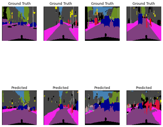
可视化一组测试结果
预测
# 每次仅取一组(16张)进行显示;(若要显示下一组,需要再迭代运行一轮以下代码)
x,y = iter(test_loader).__next__()

img = gen_images(x)
img = img.to(device).type(torch.float)
mask = gen_mask_train(y,label_dic)
mask = mask.to(device)

net.eval() # 模型切换到评估模式

# 生成预测结果
with torch.no_grad():
  y_pred = net(img)
可视化
fig = plt.figure(figsize = (10,10))

# n_images之前定义为4,代表一行4张图片;
for i in range(11,15):
  ax = fig.add_subplot(2, n_images, i-10)
  visualization = visual_label(mask[i,:,:].cpu().numpy(),labels_used)

  ax.imshow(visualization)
  ax.set_title('Ground Truth')
  ax.axis('off')

  ax = fig.add_subplot(2, n_images, i-6)
  y_test = y_pred.permute(0,2,3,1)[i,:,:,:].cpu().numpy()
  visual_test = visual_label(np.argmax(y_test,axis=2),labels_used)

  ax.imshow(visual_test)
  ax.set_title('Predicted')
  ax.axis('off')


 786
786

 被折叠的 条评论
为什么被折叠?
被折叠的 条评论
为什么被折叠?
 到【灌水乐园】发言


