Coursera | Andrew Ng (02-week-1-1.5)—为什么正则化可以减少过拟合？

该系列仅在原课程基础上部分知识点添加个人学习笔记，或相关推导补充等。如有错误，还请批评指教。在学习了 Andrew Ng 课程的基础上，为了更方便的查阅复习，将其整理成文字。因本人一直在学习英语，所以该系列以英文为主，同时也建议读者以英文为主，中文辅助，以便后期进阶时，为学习相关领域的学术论文做铺垫。- ZJ

Coursera 课程 |deeplearning.ai |网易云课堂

---

转载请注明作者和出处：ZJ 微信公众号-「SelfImprovementLab」

知乎：https://zhuanlan.zhihu.com/c_147249273

CSDN：http://blog.csdn.net/JUNJUN_ZHAO/article/details/79065804

---

1.5 Why regularization reduces overfitting

为什么正则化可以减少过拟合？

(字幕来源：网易云课堂)

**Why does regularization help with overfitting?**Why does it help with reducing variance problems?Let’s go through a couple examples to gain some intuition about how it works.So, recall that high bias, high variance, just right.and I just write pictures from our earlier video that looks something like this.Now, let’s see a fitting large and deep neural network.I know I haven’t drawn this one too large or too deep,unless you think some neural network and this currently overfitting.So you have some cost function like J of W,B equals sum of the losses.So what we did for regularization was add this extra term that penalizes the weight matrices from being too large.So that was the Frobenius norm.So why is it that shrinking the L2 norm or the Frobenius norm or the parameters might cause less overfitting?

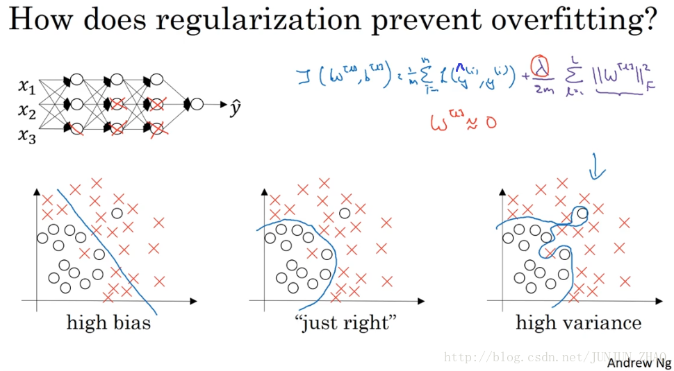
为什么正则化有利于预防过拟合呢，为什么它可以减少方差问题，我们通过两个例子来直观体会一下，左图是高偏差 右图是高方差 中间的是 Just Right，这几张图我们在前面课程中看到过，现在我们来看下这个庞大的深度拟合神经网络，我知道这张图不够大 深度也不够，但你可以想象这是一个过拟合的神经网络，这是我们的代价函数 J 含有参数 w b，等于损失总和，我们添加正则项，它可以避免数据权值矩阵过大，这就是弗罗贝尼乌斯范数，为什么压缩 L2 范数，或弗罗贝尼乌斯范数或者参数可以减少过拟合，直观上理解就是如果正则化λ设置得足够大，权重矩阵 W 被设置为接近于 0 的值。

One piece of intuition is that if you crank regularization lambda to be really, really big,they’ll be really incentivized to set the weight matrices W to be reasonably close to zero.So one piece of intuition is maybe it set the weight to be so close to zero for a lot of hidden units that’s basically zeroing out a lot of the impact of these hidden units.And if that’s the case,then this much simplified neural network becomes a much smaller neural network.In fact, it is almost like a logistic regression unit,but stacked most probably as deep.And so that will take you from this overfitting case much closer to the left to other high bias case.But hopefully there’ll be an intermediate value of lambda that results in a result closer to this just right case in the middle.But the intuition is that by cranking up lambda to be really big,they’ll set W close to zero,which in practice this isn’t actually what happens.We can think of it as zeroing out or at least reducing the impact of a lot of the hidden units so you end up with what might feel like a simpler network.They get closer and closer to as if you’re just using logistic regression.The intuition of completely zeroing out of a bunch of hidden units isn’t quite right.It turns out that what actually happens is they’ll still use all the hidden units,but each of them would just have a much smaller effect.But you do end up with a simpler network and as if you have a smaller network that is therefore less prone to overfitting.So I am not sure this intuition helps, but when you implement regularization in the program exercise,you actually see some of these variance reduction results yourself.

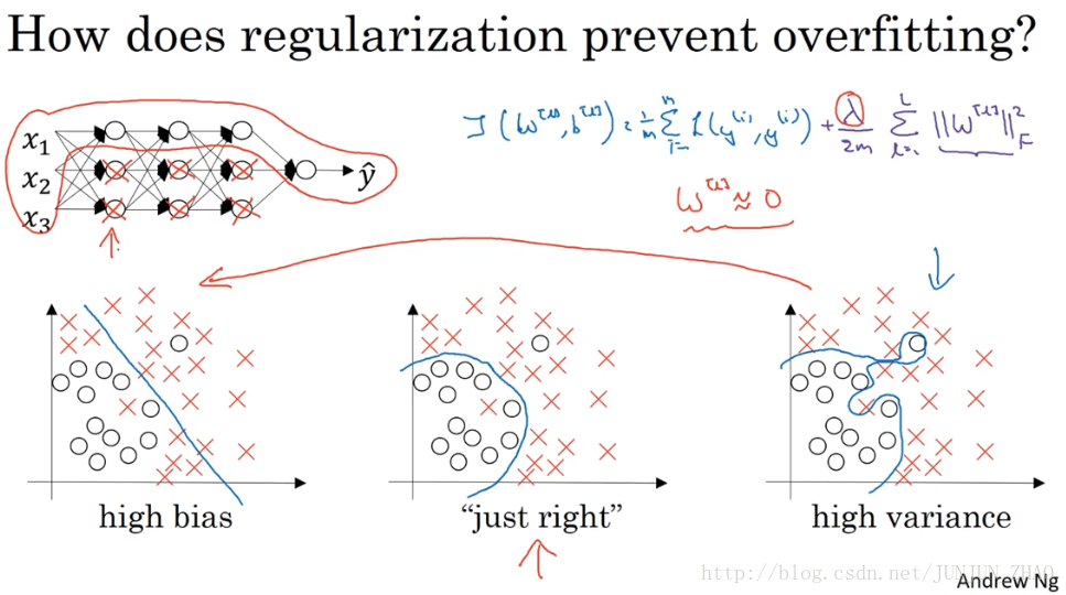
直观理解就是把多隐藏单元的权重设为 0，于是基本上消除了这些隐藏单元的许多影响，如果是这种情况，这个被大大简化了的神经网络会变成一个很小的网络，小到如同一个逻辑回归单元，可是深度却很大，它会使这个网络从过拟合的状态，更接近于左图的高偏差状态，但是 λ 会存在一个中间值，于是会有一个接近“just right”的中间状态，直观理解就是 λ 增加到足够大，W 会接近于 0，实际上是不会发生这种情况的，我们尝试消除或至少减少许多隐藏单元的影响，最终这个网络会变得更简单，这个神经网络越来越接近逻辑回归，我们直觉上认为大量隐藏单元被完全消除了 其实不然，实际上是该神经网络的所有隐藏单元依然存在，但是它们的影响变得更小了，神经网络变得更简单了，貌似这样更不容易发生过拟合，因此我不确定这个直觉经验是否有用，不过 在编程中执行正则化时，你会实际看到一些方差减少的结果。

Here’s another attempt at additional intuition for why regularization helps prevent overfitting.And for this, I’m going to assume that we’re using the tanh activation function which looks like this.This is a g of z equals tanh of z.So if that’s the case,notice that so long as Z is quite small,so if Z takes on only a smallish range of parameters, maybe around here,maybe around here, then you’re just using the linear regime of the tanh function.Is only if Z is allowed to wander up to larger values or smaller values like so,that the activation function starts to become less linear.So the intuition you might take away from this is that if lambda,the regularization parameter is large,then you have that your parameters will be relatively small,because they are penalized being large into a cos function.And so if the weights W are small then because Z is equal to W,right, and then technically is plus b,but if W tends to be very small,then Z will also be relatively small.And in particular, if Z ends up taking relatively small values,just in this whole range,then G of Z will be roughly linear.So it’s as if every layer will be roughly linear,as if it is just linear regression.And we saw in course one that if every layer is linear,then your whole network is just a linear network.And so even a very deep network,with a deep network with a linear activation functionis at the end they are only able to compute a linear function.So it’s not able to fit those very very complicated decision,very non-linear decision boundaries that allow it to really overfit right to data sets like we saw on the overfitting high variance case on the previous slide.

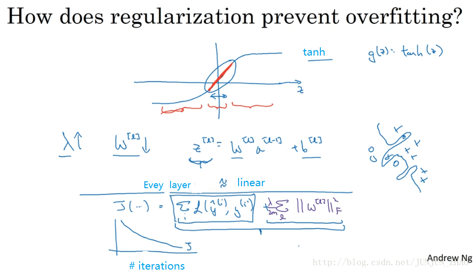
我们再来直观感受一下，正则化为什么可以预防过拟合，假设我们用的是这样的双曲激活函数，用 g(z) 表示 tanh(z)，那么我们发现，只要z 非常小，如果 z 只涉及少量参数，这里我们利用了双曲正切函数的线性状态，只要 Z 可以扩展为这样的更大值或者更小值，激活函数开始变得非线性，现在你应该摒弃这个直觉 即，如果正则参数 λ 很大，激活函数的参数会相对小，因为代价函数中的参数变大了，如果 W 很小，z 等于 w，然后再加上 b，如果 w 很小，相对来说 z 也会很小，特别是 如果 z 的值最终在这个范围内，都是相对较小的值，g(z) 大致呈线性，每层几乎都是线性的，和线性回归函数一样，第一节课我们讲过 如果每层都是线性的，那么整个网络就是一个线性网络，即使是一个非常深的深层网络，因具有线性激活函数的特征，最终我们只能计算线性函数。因此 它不适用于非常复杂的决策，以及过度拟合数据集的非线性决策边界，如同我们在上张幻灯片中看到的过度拟合高方差的情况。

So just to summarize,if the regularization parameter becomes very large,the parameters W very small,so Z will be relatively small,kind of ignoring the effects of b for now,so Z will be relatively small or,really, I should say it takes on a small range of values.And so the activation function if is tanh,say, will be relatively linear.And so your whole neural network will be computing something not too far from a big linear function which is therefore pretty simple function rather than a very complex highly non-linear function.And so is also much less able to overfit.And again, when you implement regularization for yourself in the program exercise,you’ll be able to see some of these effects yourself.Before wrapping up our def discussion on regularization,I just want to give you one implementational tip.Which is that, when implanting regularization,we took our definition of the cost function J, and we actually modifiedit by adding this extra term that penalizes the weight being too large.

总结一下，如果正则化参数变得很大，参数 W 很小，z 也会相对变小，此时忽略 b 的影响，z 会相对变小，实际上 z 的取值范围很小，这个激活函数 也就是曲线函数，会相对呈线性，整个神经网络会计算离线性函数近的值，这个线性函数非常简单，并不是一个极复杂的高度非线性函数，不会发生过拟合。大家在编程作业里实现正则化的时候，会亲眼看到这些结果，总结正规化之前，我给大家一个执行方面的小建议，在增加正则化项时，应用之前定义的代价函数 J，我们做过修改 增加了一项 目的是预防权重过大。

And so if you implement gradient descent,one of the steps to debug gradient descent is to plot the cost function J as a functionof the number of elevations of gradient descent, and you want to see thatthe cost function J decreases monotonically after every elevation of gradient descent.And if you’re implementing regularization,then please remember that J now has this new definition.If you plot the old definition of J,just this first term,then you might not see a decrease monotonically.So to debug gradient descent make sure that you’re plottingthis new definition of J that includes this second term as well.Otherwise you might not see J decrease monotonically on every single elevation.So that’s it for L two regularization which is actuallya regularization technique that I use the most in training deep learning modules.In deep learning, there is another sometimes used regularization techniquecalled dropout regularization.Let’s take a look at that in the next video.

如果你使用的是梯度下降函数，在调试梯度下降时 其中一步就是把代价函数 J 设计成这样一个函数，它代表梯度下降的调幅数量，可以看到 代价函数对于梯度下降的每个调幅都单调递减，如果你实施的是正规化函数，请牢记 J 已经有一个全新的定义，如果你用的是原函数J，也就是这第一个正则化项，你可能看不到单调递减现象，为了调试梯度下降，请务必使用新定义的J函数 它包含第二个正则化项，否则函数 J可能不会在所有调幅范围内都单调递减，这就是 L2 正则化，它是我在训练深度学习模型时最常用的一种方法，在深度学习中 还有一种方法也用到了正则化，就是 dropout 正则化，我们下节课再讲。

---

重点总结：

为什么正则化可以减小过拟合

假设下图的神经网络结构属于过拟合状态：

对于神经网络的 Cost function：

$J(w^{[1]},b^{[1]},\cdots,w^{[L]},b^{[L]})=\dfrac{1}{m}\sum\limits_{i=1}^{m}L(\hat y^{(i)},y^{(i)})+\dfrac{\lambda}{2m}\sum\limits_{l=1}^{L}||w^{[l]}||_{F}^{2}$

加入正则化项，直观上理解，正则化因子λ设置的足够大的情况下，为了使代价函数最小化，权重矩阵W就会被设置为接近于0的值。则相当于消除了很多神经元的影响，那么图中的大的神经网络就会变成一个较小的网络。

当然上面这种解释是一种直观上的理解，但是实际上隐藏层的神经元依然存在，但是他们的影响变小了，便不会导致过拟合。

数学解释：

假设神经元中使用的激活函数为 $g(z)=tanh(z)$，在加入正则化项后：

当$λ$增大，导致$W^{[l]}$减小，$Z^{[l]}=W^{[l]}a^{[l-1]}+b^{[l]}$便会减小，由上图可知，在 z 较小的区域里，$tanh(z)$函数近似线性，所以每层的函数就近似线性函数，整个网络就成为一个简单的近似线性的网络，从而不会发生过拟合。

参考文献：

[1]. 大树先生.吴恩达Coursera深度学习课程 DeepLearning.ai 提炼笔记（2-1）– 深度学习的实践方面

---

PS: 欢迎扫码关注公众号：「SelfImprovementLab」！专注「深度学习」，「机器学习」，「人工智能」。以及 「早起」，「阅读」，「运动」，「英语 」「其他」不定期建群 打卡互助活动。