Coursera | Andrew Ng (02-week-1-1.9)—归一化输入

该系列仅在原课程基础上部分知识点添加个人学习笔记，或相关推导补充等。如有错误，还请批评指教。在学习了 Andrew Ng 课程的基础上，为了更方便的查阅复习，将其整理成文字。因本人一直在学习英语，所以该系列以英文为主，同时也建议读者以英文为主，中文辅助，以便后期进阶时，为学习相关领域的学术论文做铺垫。- ZJ

Coursera 课程 |deeplearning.ai |网易云课堂

---

转载请注明作者和出处：ZJ 微信公众号-「SelfImprovementLab」

知乎：https://zhuanlan.zhihu.com/c_147249273

CSDN：http://blog.csdn.net/junjun_zhao/article/details/79074200

---

1.9 Normalizing inputs (正则化输入)

(字幕来源：网易云课堂)

When training a neural network, one of the techniques that will speed up your training is if you normalize your inputs. Let’s see what that means. Let’s see if we have a training sets with two input features. So the input features x are two dimensional, and here’s a scatter plot of your training set. Normalizing your inputs corresponds to two steps. The first is to subtract out or to zero out the mean. So you set μ = 1/m sum over I of $X^{(i)}$. So this is a vector, and then X gets set as X- μ for every training example,so this means you just move the training set until it has 0 mean.

训练神经网络 其中一个加速训练的方法就是 ，归一化输入，我们来了解一下，假设我们有一个训练集 它有两个输入特征，所以输入特征 x 是二维的，这是数据集的散点图，归一化输入需要两个步骤，第一步是零均值化， μ 等于1/m 乘以 $X^{(i)}$ 从 i=1 到 m 之和，它是一个向量 X 等于每个训练数据 x 减去 μ ，意思是移动训练集 直到它完成零均值化 。

And then the second step is to normalize the variances. So notice here that the feature X1 has a much larger variance than the feature X2 here. So what we do is set σ=1/m sum of $X^{(i)}**2$. I guess this is a element y squaring. And so now sigma squared is a vector with the variances of each of the features, and notice we’ve already subtracted out the mean, so $X^{(i)}$ squared, element y squared is just the variances. And you take each example and divide it by this vector sigma squared. And so in pictures, you end up with this, where now the variance of X1 and X2 are both equal to one. And one tip, if you use this to scale your training data, then use the same mu and sigma squared to normalize your test set, right? In particular, you don’t want to normalize the training set and the test set differently. Whatever this value is and whatever this value is, use them in these two formulas, so that you scale your test set in exactly the same way, rather than estimating mu and sigma squared separately on your training set and test set. Because you want your data, both training and test examples, to go through the same transformation defined by the same mu and sigma squared calculated on your training data.

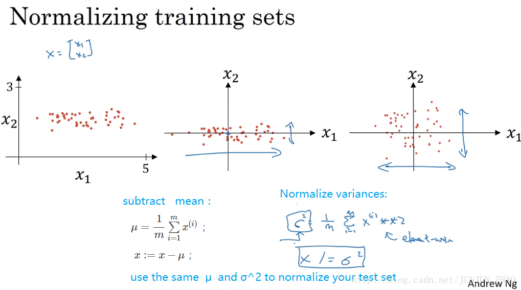
第二步是归一化方差，注意 特征 x1 的方差比特征 x2 的方差要大得多，我们要做的是给 σ 赋值 $\sigma^{2} = \dfrac{1}{m}\sum\limits_{i=1}^{m}x^{(i)^{2}}$， 这是节点 y 的平方， $σ^2$是一个向量 它的每个特征都有方差，注意 我们已经完成零值均化， $X^{{(i)}^2}$ 元素 $y^2$ 就是方差，我们把所有数据都除以向量 $σ^2$，图片最后变成这样，x1 和 x2 的方差都等于 1，提示一下 如果你用它来调整训练数据，那么用相同的 μ 和 $σ^2$来归一化测试集， 尤其是 你不希望训练集和测试集的归一化有所不同，不论 μ 的值是什么 也不论 $σ^2$的值是什么 ,这两个公式中都会用到它们，所以你要用同样的方法调整测试集，而不是在训练集和测试集上分别预估 μ 和 $σ^2$，因为我们希望不论是训练数据还是测试数据，都是通过相同 μ 和 $σ^2$定义的相同数据转换，其中 μ 和 $σ^2$是由训练集数据计算得来的。

So, why do we do this? Why do we want to normalize the input features? Recall that a cost function is defined as written on the top right. It turns out that if you use unnormalized input features, it’s more likely that your cost function will look like this, it’s a very squished out bowl, very elongated cost function, where the minimum you’re trying to find is maybe over there. But if your features are on very different scales, say the feature X1 ranges from 1 to 1000, and the feature X2 ranges from 0 to 1, then it turns out that the ratio or the range of values for the parameters w1 and w2 will end up taking on very different values. And so maybe these axes should be w1 and w2, but with intuition I’ll plot w and b, then your cost function can be a very elongated bowl like that. So if you part the contours of this function, you can have a very elongated function like that. Whereas if you normalize the features, then your cost function will on average look more symmetric.

我们为什么要这么做呢，为什么我们想归一化输入特征，回想一下右上角所定义的代价函数，如果你使用非归一化的输入特征，代价函数将会像这样，这是一个非常细长狭窄的代价函数，你要找的最小值应该在这里，但如果特征值在不同范围，假如 x1 取值范围从 1 到 1000，特征 x2 的取值范围从 0 到 1，结果是参数 w1 和 w2 值的范围或比率，将会非常不同，这些数据轴应该是 w1 和 w2 但直观理解 我标记为 w 和 b，代价函数就有点像狭长的碗一样，如果你能画出该函数的部分轮廓，它会是这样一个狭长的函数，然而如果你归一化特征，代价函数平均起来看更对称。

And if you’re running gradient descent on the cost function like the one on the left, then you might have to use a very small learning rate, because if you’re here, that gradient descent might need a lot of steps to oscillate back and forth before it finally finds its way to the minimum. Whereas if you have a more spherical contours, then wherever you start, gradient descent can pretty much go straight to the minimum. You can take much larger steps with gradient descent rather than needing to oscillate around like the picture on the left. Of course in practice w is a high-dimensional vector, and so trying to plot this in 2D doesn’t convey all the intuitions correctly. But the rough intuition that your cost function will be more round and easier to optimize when your features are all on similar scales, not from 1 to 1000, zero to one, but mostly from -1 to 1 or of about similar variances of each other. That just makes your cost function J easier and faster to optimize. In practice if one feature, say X1, ranges from zero to one, and X2 ranges from -1 to 1, and X3 ranges from one to two,these are fairly similar ranges, so this will work just fine. It’s when they’re on dramatically different ranges like ones from 1 to a 1000, and the another from 0 to 1, that that really hurts your optimization algorithm. But by just setting all of them to a 0 mean and say, variance 1, like we did in the last slide, that just guarantees that all your features on a similar scale and will usually help your learning algorithm run faster.

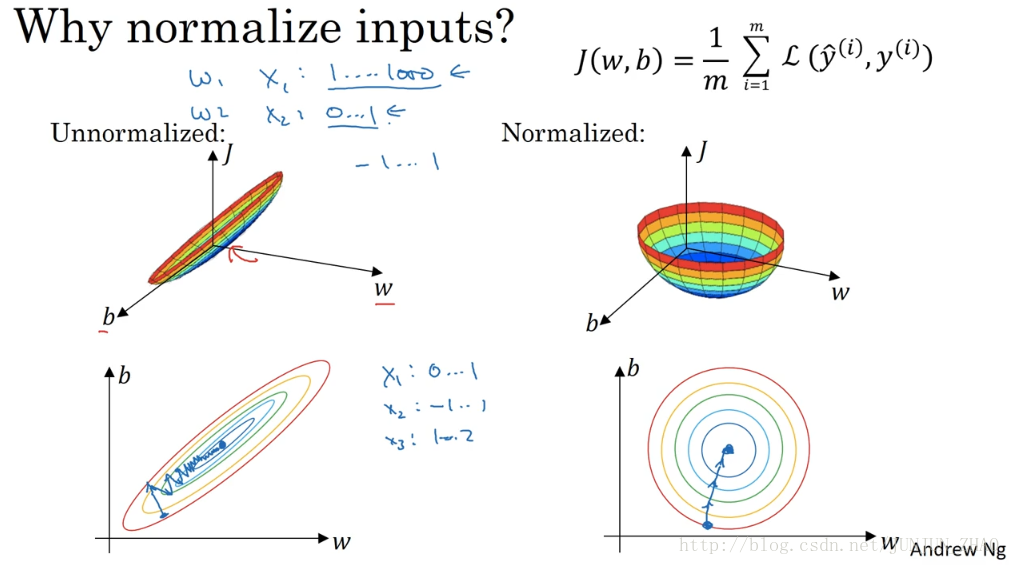
如果你在左图这样的代价函数上运行梯度下降法，你必须使用一个非常小的学习比率，因为如果是在这个位置 梯度下降法可能需要多次迭代过程，直到最后找到最小值，但如果函数是一个更圆的球形轮廓 那么不论从哪个位置开始，梯度下降法都能够更直接地找到最小值，你可以在梯度下降法中使用较大步长，而不需要像在左图中那样反复执行，当然 实际上 w 是一个高维向量，因此用二维绘制 w 并不能正确地传达直观理解，但总的直观理解是代价函数会更圆一些 而且更容易优化，前提是特征都在相似范围内，而不是从 1 到 1000, 0 到 1 的范围，而是在-1到1范围内或相似偏差，这使得代价函数 J 优化起来更简单更快速，实际上 如果假设特征 x1 范围在 0-1之间，x2 范围在 -1-1之间 x3 范围在 1-2 之间，它们是相似范围 所以会表现得很好 ，当它们在非常不同的取值范围内 如其中一个从1 到 1000，另一个从 0 到 1 这对优化算法非常不利，但是仅将它们设置为均化零值 假设方差为 1，就像上一张幻灯片里设定的那样 确保所有特征都在相似范围内，通常可以帮助学习算法运行得更快。

So, if your input features came from very different scales, maybe some features are from 0 to 1, some from 1 to 1000, then it’s important to normalize your features. If your features came in on similar scales, then this step is less important, although performing this type of normalization pretty much never does any harm, so I’ll often do it anyway if I’m not sure whether or not it will help with speeding up training for your algorithm. So that’s it for normalizing your input features. Next, let’s keep talking about ways to speed up the training of your neural network.

所以如果输入特征处于不同范围内，可能有些特征值从 0 到 1 有些从 1 到 1000，那么归一化特征值就非常重要了，如果特征值处于相似范围内 那么归一化就不是很重要了，执行这类归一化并不会产生什么危害，我经常会做归一化处理，虽然我不确定它能否提高训练或算法速度，这就是归一化输入特征，下节课我们将继续探讨提升神经网络训练速度的方法。

---

重点总结：

归一化输入

对数据集特征 x1,x2 归一化的过程：

• 计算每个特征所有样本数据的均值：$\mu = \dfrac{1}{m}\sum\limits_{i=1}^{m}x^{(i)}$；
• 减去均值得到对称的分布：$x : =x-\mu$；
• 归一化方差：$\sigma^{2} = \dfrac{1}{m}\sum\limits_{i=1}^{m}x^{(i)^{2}}$, $x = x/\sigma^{2}$

使用归一化的原因：

由图可以看出不使用归一化和使用归一化前后 Cost function 的函数形状会有很大的区别。

在不使用归一化的代价函数中，如果我们设置一个较小的学习率，那么很可能我们需要很多次迭代才能到达代价函数全局最优解；

如果使用了归一化，那么无论从哪个位置开始迭代，我们都能以相对很少的迭代次数找到全局最优解。

参考文献：

[1]. 大树先生.吴恩达Coursera深度学习课程 DeepLearning.ai 提炼笔记（2-1）– 深度学习的实践方面

---

PS: 欢迎扫码关注公众号：「SelfImprovementLab」！专注「深度学习」，「机器学习」，「人工智能」。以及 「早起」，「阅读」，「运动」，「英语 」「其他」不定期建群 打卡互助活动。