T4猴痘病识别

• 🍨 本文为🔗365天深度学习训练营 中的学习记录博客
• 🍖 原作者：K同学啊 | 接辅导、项目定制
• 🚀 文章来源：K同学的学习圈子
  本文采用Tensorflow的框架，进行猴痘病图像的检测识别，数据由K同学提供。

一 前期准备

1. 设置GPU

在anaconda prompt中新建名称为tensorflow_cpu的环境，并安装tensorflow，matplotlib的包。同时脚本代码为ipy文件，需要安装ipykernel。

conda create -n tensorflow_cpu python=3.6
conda activate tensorflow_cpu
pip install tensorflow
pip install matplotlib
pip install ipykernel

输出使用的电脑配置。

from datetime import datetime
import sys
import matplotlib
print("Current time:", datetime.today())
print("Python version:", sys.version)
print("Tensorflow version", tf.__version__)
print("Matplotlib version", matplotlib.__version__)
gpus = tf.config.list_physical_devices("GPU")
if gups:
    gpu0 = gpus[0]
    tf.config.experimental.set_memory_growth(gpu0, True)
    tf.config.set_visible_devices([gpu0],"GPU")
    print("Device: GPU")
else:
    print("Device: CPU")

Current time: 2023-11-17 20:14:33.985956
Python version: 3.6.15 (default, Dec  3 2021, 18:25:24) [MSC v.1916 64 bit (AMD64)]
Tensorflow version 2.6.2
Matplotlib version 3.3.4
Device: CPU

2. 导入数据并查看数据

导入数据并展示示例图片，图片总数为2142。

import os, PIL, pathlib
# data_dir = './Monkeypox/'
data_dir = "../T4data/"
data_dir = pathlib.Path(data_dir)
image_count = len(list(data_dir.glob('*/*.jpg')))
print("图片总数为：",image_count)
Monkeypox = list(data_dir.glob('Monkeypox/*.jpg'))
PIL.Image.open(str(Monkeypox[0]))

二、数据预处理

1. 加载数据

划分训练集和测试集，其中训练集数据为900张，测试集数据为225张。

train_ds = tf.keras.preprocessing.image_dataset_from_directory(
    data_dir,
    validation_split=0.2,
    subset="training",
    seed=123,
    image_size=(img_height, img_width),
    batch_size=batch_size)
val_ds = tf.keras.preprocessing.image_dataset_from_directory(
    data_dir,
    validation_split=0.2,
    subset="validation",
    seed=123,
    image_size=(img_height, img_width),
    batch_size=batch_size)

2. 可视化

import matplotlib.pyplot as plt
plt.figure(figsize=(20, 10))
for images, labels in train_ds.take(1):
    for i in range(20):
        ax = plt.subplot(5, 10, i + 1)
        plt.imshow(images[i].numpy().astype("uint8"))
        plt.title(class_names[labels[i]])      
        plt.axis("off")

3. 配置数据集

AUTOTUNE = tf.data.AUTOTUNE
train_ds = train_ds.cache().shuffle(1000).prefetch(buffer_size=AUTOTUNE)
val_ds = val_ds.cache().prefetch(buffer_size=AUTOTUNE)

二 构建网络模型

1. 搭建模型

构建三层卷积、两层全连接的神经网络。

num_classes = 2
from tensorflow.keras import layers, models
model = models.Sequential([
    layers.experimental.preprocessing.Rescaling(1./255, input_shape=(img_height, img_width, 3)),
    
    layers.Conv2D(16, (3, 3), activation='relu', input_shape=(img_height, img_width, 3)), # 卷积层1，卷积核3*3  
    layers.AveragePooling2D((2, 2)),               # 池化层1，2*2采样
    layers.Conv2D(32, (3, 3), activation='relu'),  # 卷积层2，卷积核3*3
    layers.AveragePooling2D((2, 2)),               # 池化层2，2*2采样
    layers.Dropout(0.3),  
    layers.Conv2D(64, (3, 3), activation='relu'),  # 卷积层3，卷积核3*3
    layers.Dropout(0.3),  
    
    layers.Flatten(),                       # Flatten层，连接卷积层与全连接层
    layers.Dense(128, activation='relu'),   # 全连接层，特征进一步提取
    layers.Dense(num_classes)               # 输出层，输出预期结果
])
model.summary()  # 打印网络结构

模型结构如下所示

Model: "sequential"
_________________________________________________________________
Layer (type)                 Output Shape              Param #   
=================================================================
rescaling (Rescaling)        (None, 224, 224, 3)       0         
_________________________________________________________________
conv2d (Conv2D)              (None, 222, 222, 16)      448       
_________________________________________________________________
average_pooling2d (AveragePo (None, 111, 111, 16)      0         
_________________________________________________________________
conv2d_1 (Conv2D)            (None, 109, 109, 32)      4640      
_________________________________________________________________
average_pooling2d_1 (Average (None, 54, 54, 32)        0         
_________________________________________________________________
dropout (Dropout)            (None, 54, 54, 32)        0         
_________________________________________________________________
conv2d_2 (Conv2D)            (None, 52, 52, 64)        18496     
_________________________________________________________________
dropout_1 (Dropout)          (None, 52, 52, 64)        0         
_________________________________________________________________
flatten (Flatten)            (None, 173056)            0         
_________________________________________________________________
dense (Dense)                (None, 128)               22151296  
_________________________________________________________________
dense_1 (Dense)              (None, 2)                 258       
...
Total params: 22,175,138
Trainable params: 22,175,138
Non-trainable params: 0

三 编译

# 设置优化器
opt = tf.keras.optimizers.Adam(learning_rate=1e-4)
model.compile(optimizer=opt,
              loss=tf.keras.losses.SparseCategoricalCrossentropy(from_logits=True),
              metrics=['accuracy'])

四 训练模型

from tensorflow.keras.callbacks import ModelCheckpoint
epochs = 50
checkpointer = ModelCheckpoint('best_model.h5',
                                monitor='val_accuracy',
                                verbose=1,
                                save_best_only=True,
                                save_weights_only=True)
history = model.fit(train_ds,
                    validation_data=val_ds,
                    epochs=epochs,
                    callbacks=[checkpointer])

训练过程如下

Epoch 1/50
54/54 [==============================] - 34s 598ms/step - loss: 0.7086 - accuracy: 0.5659 - val_loss: 0.7388 - val_accuracy: 0.5374

Epoch 00001: val_accuracy improved from -inf to 0.53738, saving model to best_model.h5
Epoch 2/50
54/54 [==============================] - 31s 579ms/step - loss: 0.6620 - accuracy: 0.6149 - val_loss: 0.6695 - val_accuracy: 0.6192

Epoch 00002: val_accuracy improved from 0.53738 to 0.61916, saving model to best_model.h5
Epoch 3/50
54/54 [==============================] - 28s 513ms/step - loss: 0.6117 - accuracy: 0.6669 - val_loss: 0.5920 - val_accuracy: 0.6799

Epoch 00003: val_accuracy improved from 0.61916 to 0.67991, saving model to best_model.h5
Epoch 4/50
54/54 [==============================] - 27s 507ms/step - loss: 0.5655 - accuracy: 0.7130 - val_loss: 0.6273 - val_accuracy: 0.6495

Epoch 00004: val_accuracy did not improve from 0.67991
Epoch 5/50
54/54 [==============================] - 29s 533ms/step - loss: 0.5382 - accuracy: 0.7305 - val_loss: 0.5694 - val_accuracy: 0.7126

Epoch 00005: val_accuracy improved from 0.67991 to 0.71262, saving model to best_model.h5
Epoch 6/50
54/54 [==============================] - 29s 545ms/step - loss: 0.5045 - accuracy: 0.7509 - val_loss: 0.4730 - val_accuracy: 0.7757

Epoch 00006: val_accuracy improved from 0.71262 to 0.77570, saving model to best_model.h5
Epoch 7/50
...
Epoch 50/50
54/54 [==============================] - 29s 542ms/step - loss: 0.0490 - accuracy: 0.9825 - val_loss: 0.5180 - val_accuracy: 0.8668

Epoch 00050: val_accuracy did not improve from 0.89252

五 预测

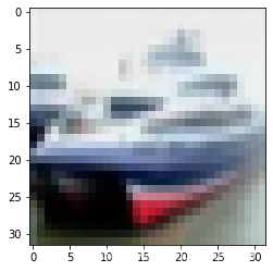
plt.imshow(test_images[1])
import numpy as np
pre = model.predict(test_images)
print(class_names[np.argmax(pre[1])])
ship

![在这里插入图片描述](https://img-blog.csdnimg.cn/cfebf30b0b254833a5c12e238fa72ca4.png#pic_center

六 模型评估

acc = history.history['accuracy']
val_acc = history.history['val_accuracy']

loss = history.history['loss']
val_loss = history.history['val_loss']

epochs_range = range(epochs)

plt.figure(figsize=(12, 4))
plt.subplot(1, 2, 1)
plt.plot(epochs_range, acc, label='Training Accuracy')
plt.plot(epochs_range, val_acc, label='Validation Accuracy')
plt.legend(loc='lower right')
plt.title('Training and Validation Accuracy')

plt.subplot(1, 2, 2)
plt.plot(epochs_range, loss, label='Training Loss')
plt.plot(epochs_range, val_loss, label='Validation Loss')
plt.legend(loc='upper right')
plt.title('Training and Validation Loss')
plt.show()

采用CPU训练速度已经可见有些慢。下一步需要配置一下gpu环境。