Python数据分析之NumPy（1）——NumPy快速入门笔记：用一篇文章快速解最核心的NumPy知识

最新推荐文章于 2023-07-12 06:48:44 发布

置顶 Robin_Pi

最新推荐文章于 2023-07-12 06:48:44 发布

阅读量530

点赞数 1

分类专栏：机器学习之路 Numpy-Pandas-Matplotlib # Python 文章标签： python 数据分析 numpy 机器学习大数据

本文链接：https://blog.csdn.net/Robin_Pi/article/details/103533836

版权

Python 同时被 3 个专栏收录

85 篇文章 11 订阅

订阅专栏

机器学习之路

27 篇文章 2 订阅

订阅专栏

Numpy-Pandas-Matplotlib

26 篇文章 2 订阅

订阅专栏

1. 几个重要概念

1.1 NumPy array （NumPy数组）

NumPy’s main object is the homogeneous multidimensional array. It
is a table of elements (usually numbers), all of the same type,
indexed by a tuple of non-negative integers.

注意一点：array中的元素是相同的类型
（以下基本用“数组”代替“NumPy数组”）

1.2 one axis/ axes（轴）

In NumPy dimensions are called axes.

在NumPy中，维度被称为轴。
很重要的概念。
在这里插入图片描述
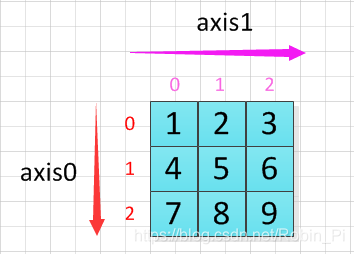
在下面这个例子中，数组有两轴：
第一个轴的长度是2，第二个轴的长度是1。

[[ 1., 0., 0.],
 [ 0., 1., 2.]]

axis=0 即行变化的方向；axis=1 即列变化的方向。

记住轴的这些概念，后面会说到数组的合并，会再次用到它们。

1.3 element（元素）

number of element = length of a axis
一个轴元素的个数即是这个轴的长度。

1.4 ndarray

NumPy’s array class is called ndarray.
NumPy中的数组类被称作ndarray。

注意：numpy.array ≠ array.array （只有一维）
ndarray 重要的属性如下：

ndarray.ndim
轴的数量或数组的维度数量
ndarray.shape
数组的（形状）大小，也就是：用元组来表示每个维度上元素的数量
ndarray.size
数组所含的元素总数（所有轴）
ndarray.dtype
描述数组中元素类型的对象

除了可以使用python类型来定义数组元素的类型，NumPy还提供了它自己的：
numpy.int32,、numpy.int16、和numpy.float64
ndarray.itemsize
所含元素的字节大小
例如， float64 的 itemsize 是 8 (=64/8), 而 complex32 的 itemsize 是4 (=32/8)。实际上，相当于是 ndarray.dtype.itemsize.

一个例子：

>>> import numpy as np
>>> a = np.arange(15).reshape(3, 5)
>>> a
array([[ 0,  1,  2,  3,  4],
       [ 5,  6,  7,  8,  9],
       [10, 11, 12, 13, 14]])
>>> a.shape
(3, 5)
>>> a.ndim
2
>>> a.dtype.name
'int64'
>>> a.itemsize
8
>>> a.size
15
>>> type(a)
<type 'numpy.ndarray'>
>>> b = np.array([6, 7, 8])
>>> b
array([6, 7, 8])
>>> type(b)
<type 'numpy.ndarray'>

2. NumPy 的一些基本用法

2.1 创建NumPy数组

使用使用 numpy.array() 函数 + 简单的python 列表/元组快速创建

>>> import numpy as np
>>> a = np.array([2,3,4])
>>> a
array([2, 3, 4])
>>> a.dtype
dtype('int64')
>>> b = np.array([1.2, 3.5, 5.1])
>>> b.dtype
dtype('float64')

>>> c = np.array( [ [1,2], [3,4] ], dtype=complex ) # 也可以自定义元素数据类型
>>> c
array([[ 1.+0.j,  2.+0.j],
       [ 3.+0.j,  4.+0.j]])

zeros()、ones()、empty()
由于有很大一部分是这样的情况：数组的元素是不知道的，但它的形状是知道的。所以NumPy提供了一些便利的函数：

>>> np.zeros( (3,4) )
array([[ 0.,  0.,  0.,  0.],
       [ 0.,  0.,  0.,  0.],
       [ 0.,  0.,  0.,  0.]])
>>> np.ones( (2,3,4), dtype=np.int16 )                # dtype can also be specified
array([[[ 1, 1, 1, 1],
        [ 1, 1, 1, 1],
        [ 1, 1, 1, 1]],
       [[ 1, 1, 1, 1],
        [ 1, 1, 1, 1],
        [ 1, 1, 1, 1]]], dtype=int16)
>>> np.empty( (2,3) )                                 # uninitialized, output may vary
array([[  3.73603959e-262,   6.02658058e-154,   6.55490914e-260],
       [  5.30498948e-313,   3.14673309e-307,   1.00000000e+000]])

注意：

np.ones(shape, dtype=None, order=‘C’)，其中的 shape参数，是要带括号的！！
看下面的小例子：

print(np.ones(3))
[1. 1. 1.]

print(np.ones(3,3))
TypeError: data type not understood

print(np.ones((3,3)))
[[1. 1. 1.]
 [1. 1. 1.]
 [1. 1. 1.]]

arange() 和 linspace()

np.arange([start,] stop[, step,], dtype=None)
创建一个固定区间（包括stop）的、数值序列的数组（类似python的 range 函数）；
np.linspace(start, stop, num=50)
生成固定区间（包括stop）的、包含固定个数元素的数组，默认个数为50。

>>> from numpy import pi
>>> np.linspace( 0, 2, 9 )                 # 9 numbers from 0 to 2
array([ 0.  ,  0.25,  0.5 ,  0.75,  1.  ,  1.25,  1.5 ,  1.75,  2.  ])
>>> x = np.linspace( 0, 2*pi, 100 )        # useful to evaluate function at lots of points
>>> f = np.sin(x)

2.2 打印数组

有几个点需要注意：

the last axis is printed from left to right,
the second-to-last is printed from top to bottom,
the rest are also printed from top to bottom, with each slice separated from the next by an empty line.

其实，只需这样理解即可：
一维数组打印出来是以行（row）为显示；
二维数组即是平面的矩阵（装着数组的列表）；
三维数组即是装着矩阵的列表。

>>> a = np.arange(6)                         # 1d array
>>> print(a)
[0 1 2 3 4 5]
>>>
>>> b = np.arange(12).reshape(4,3)           # 2d array
>>> print(b)  
[[ 0  1  2]
 [ 3  4  5]
 [ 6  7  8]
 [ 9 10 11]]
>>>
>>> c = np.arange(24).reshape(2,3,4)         # 3d array
>>> print(c)  
[[[ 0  1  2  3]
  [ 4  5  6  7]
  [ 8  9 10 11]]
 [[12 13 14 15]
  [16 17 18 19]
  [20 21 22 23]]]

上面的a、b和c分别可以理解为：
一行（维）数组、4个一维数组和2个3x4的矩阵

reshape()返回一个更改了形状的数组，后面也会讲到。

>>> print(np.arange(10000))
[   0    1    2 ..., 9997 9998 9999]
>>>
>>> print(np.arange(10000).reshape(100,100))
[[   0    1    2 ...,   97   98   99]
 [ 100  101  102 ...,  197  198  199]
 [ 200  201  202 ...,  297  298  299]
 ...,
 [9700 9701 9702 ..., 9797 9798 9799]
 [9800 9801 9802 ..., 9897 9898 9899]
 [9900 9901 9902 ..., 9997 9998 9999]]

一个小知识点：
想要显示完整的结果可以使用打印中的可选项：set_printoptions。

>>> np.set_printoptions(threshold=sys.maxsize)       # sys module should be imported

2.3 基本操作

Arithmetic operators on arrays apply elementwise. A new array is created and filled with the result.
需要记住的一点是：NumPy数组是

四则运算 + - * /
注意：使用条件是形状相同的两个矩阵：

>>> A = np.array( [[1,1],
...             [0,1]] )
>>> B = np.array( [[2,0],
...             [3,4]] )
>>> A * B                       # elementwise product

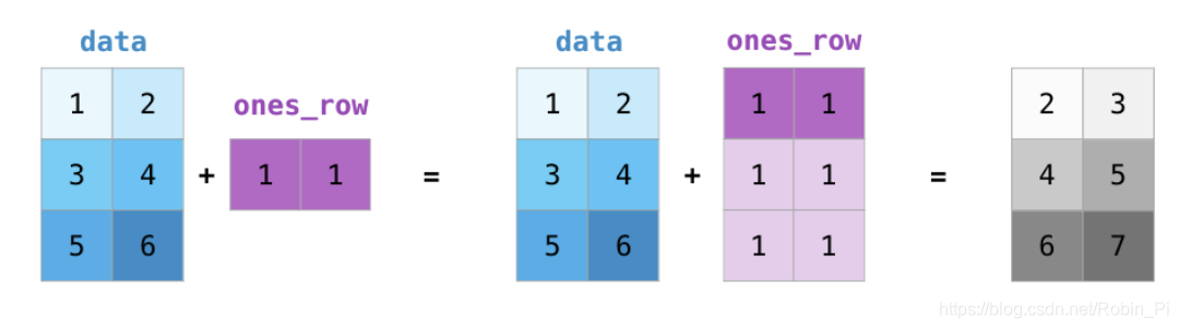
如果是一个矩阵和一个一维的向量，这种情况，NumPy会使用它的广播机制，如下图：
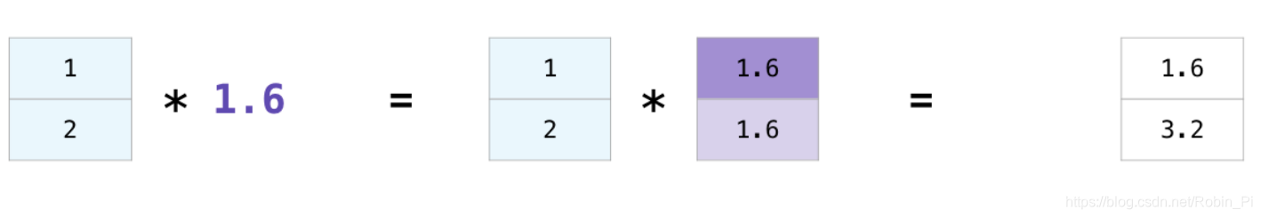
在这里插入图片描述数组的数乘同样这样理解：

点乘
数组点乘有两种表示，可以用 dot()函数或者方法，也可以使用 @ （python＞＝3.5）

>>> A = np.array( [[1,1],
...             [0,1]] )
>>> B = np.array( [[2,0],
...             [3,4]] )
>>> A * B                       # elementwise product
array([[2, 0],
       [0, 4]])
>>> A @ B                       # matrix product
array([[5, 4],
       [3, 4]])
>>> A.dot(B)                    # another matrix product
array([[5, 4],
       [3, 4]])

注意：

* 是 elementwise，跟dot()函数和@不同： A*B ≠ A.dot(B) or A @ B
一些操作，比如 += 和 *= 是在原数组上进行修改而不是创建一个新的数组。

>>> a = np.ones((2,3), dtype=int)
>>> b = np.random.random((2,3))
>>> a *= 3
>>> a
array([[3, 3, 3],
       [3, 3, 3]])
>>> b += a
>>> b
array([[ 3.417022  ,  3.72032449,  3.00011437],
       [ 3.30233257,  3.14675589,  3.09233859]])
>>> a += b                  # b is not automatically converted to integer type
Traceback (most recent call last):
  ...
TypeError: Cannot cast ufunc add output from dtype('float64') to dtype('int64') with casting rule 'same_kind'

当不同元数类型的数组进行运算时，其结果会“选择”更广的或者更精确的那种（类型）——被称作upcasting。

>>> a = np.ones(3, dtype=np.int32)
>>> b = np.linspace(0,pi,3)
>>> b.dtype.name
'float64'
>>> c = a+b
>>> c
array([ 1.        ,  2.57079633,  4.14159265])
>>> c.dtype.name
'float64'
>>> d = np.exp(c*1j)`在这里插入代码片`
>>> d
array([ 0.54030231+0.84147098j, -0.84147098+0.54030231j,
       -0.54030231-0.84147098j])
>>> d.dtype.name
'complex128'

一元操作：sum()、min()、max()

这些操作是ndarray 类中的方法。

>>> a = np.random.random((2,3))
>>> a
array([[ 0.18626021,  0.34556073,  0.39676747],
       [ 0.53881673,  0.41919451,  0.6852195 ]])
>>> a.sum()
2.5718191614547998
>>> a.min()
0.1862602113776709
>>> a.max()
0.6852195003967595

除此之外，在其它形状的数组中，可以指定需要计算的那个轴的，对上面的数组进行操作：

>>> b = np.arange(12).reshape(3,4)
>>> b
array([[ 0,  1,  2,  3],
       [ 4,  5,  6,  7],
       [ 8,  9, 10, 11]])
>>>
>>> b.sum(axis=0)                            # sum of each column
array([12, 15, 18, 21])
>>>
>>> b.min(axis=1)                            # min of each row
array([0, 4, 8])
>>>
>>> b.cumsum(axis=1)                         # cumulative sum along each row
array([[ 0,  1,  3,  6],
       [ 4,  9, 15, 22],
       [ 8, 17, 27, 38]])

2.4 通用函数

一些常见的数学函数，例如sin、cos和exp，还有sqrt、add等，在NumPy中被称为“universal functions”(ufunc).这些函数，依旧是按照数组的元素来进行操作，并产生一个数组作为结果。

>>> B = np.arange(3)
>>> B
array([0, 1, 2])
>>> np.exp(B)
array([ 1.        ,  2.71828183,  7.3890561 ])
>>> np.sqrt(B)
array([ 0.        ,  1.        ,  1.41421356])
>>> C = np.array([2., -1., 4.])
>>> np.add(B, C)
array([ 2.,  0.,  6.])

2.5 索引、切片和迭代

一维数组

类似列表以及其他python序列：

>>> a = np.arange(10)**3
>>> a
array([  0,   1,   8,  27,  64, 125, 216, 343, 512, 729])
>>> a[2]
8
>>> a[2:5]
array([ 8, 27, 64])
>>> a[:6:2] = -1000    # equivalent to a[0:6:2] = -1000; from start to position 6, exclusive, set every 2nd element to -1000
>>> a
array([-1000,     1, -1000,    27, -1000,   125,   216,   343,   512,   729])
>>> a[ : :-1]                                 # reversed a
array([  729,   512,   343,   216,   125, -1000,    27, -1000,     1, -1000])
>>> for i in a:
...     print(i**(1/3.))
...
nan
1.0
nan
3.0
nan
5.0
6.0
7.0
8.0
9.0

注意：
a[:6:2] = -1000 相当于 a[0:6:2] = -1000
每隔两个元素，将索引从0到6 位置的元素的值设置为指定的-1000

多维数组
多维数组每一个轴对应一个索引，它们之间用元组表示，用逗号隔开。

>>> def f(x,y):
...     return 10*x+y
...
>>> b = np.fromfunction(f,(5,4),dtype=int)
>>> b
array([[ 0,  1,  2,  3],
       [10, 11, 12, 13],
       [20, 21, 22, 23],
       [30, 31, 32, 33],
       [40, 41, 42, 43]])
>>> b[2,3]
23
>>> b[0:5, 1]                       # each row in the second column of b
array([ 1, 11, 21, 31, 41])
>>> b[ : ,1]                        # equivalent to the previous example
array([ 1, 11, 21, 31, 41])
>>> b[1:3, : ]                      # each column in the second and third row of b
array([[10, 11, 12, 13],
       [20, 21, 22, 23]])

如果索引的数量于数组轴的数量，则缺失的位置，用：来代替，即表示全部的切片。

>>> b[-1]                                  # the last row. Equivalent to b[-1,:]
array([40, 41, 42, 43])

3. 操纵数组的形状

改变数组的形状大小
np.ravel()
np.reshape()
np.T
np. reseize()

>>> a = np.floor(10*np.random.random((3,4)))
>>> a
array([[ 2.,  8.,  0.,  6.],
       [ 4.,  5.,  1.,  1.],
       [ 8.,  9.,  3.,  6.]])
>>> a.shape
(3, 4)

>>> a.ravel()  # returns the array, flattened
array([ 2.,  8.,  0.,  6.,  4.,  5.,  1.,  1.,  8.,  9.,  3.,  6.])
>>> a.reshape(6,2)  # returns the array with a modified shape
array([[ 2.,  8.],
       [ 0.,  6.],
       [ 4.,  5.],
       [ 1.,  1.],
       [ 8.,  9.],
       [ 3.,  6.]])
>>> a.T  # returns the array, transposed
array([[ 2.,  4.,  8.],
       [ 8.,  5.,  9.],
       [ 0.,  1.,  3.],
       [ 6.,  1.,  6.]])
>>> a.T.shape
(4, 3)
>>> a.shape
(3, 4)

注意点：
①reshape()中的参数-1，表示该轴的大小自动计算（不需要我们自己给出）
②resize和reshape的区别
reshape()不改变原数组，是返回一个新的数组；
resize()是直接修改原数组

>>> a
array([[ 2.,  8.,  0.,  6.],
       [ 4.,  5.,  1.,  1.],
       [ 8.,  9.,  3.,  6.]])
>>> a.resize((2,6))
>>> a
array([[ 2.,  8.,  0.,  6.,  4.,  5.],
       [ 1.,  1.,  8.,  9.,  3.,  6.]])

>>> a.reshape(3,-1)
array([[ 2.,  8.,  0.,  6.],
       [ 4.,  5.,  1.,  1.],
       [ 8.,  9.,  3.,  6.]])

③上面四个命令，只有resize了改变了原来的数组，其它都只是返回一个被修改了的数组。

数组合并

通过沿着不同的轴向，数组有着不同的合并方式：vstack()代表vertical stack，沿着竖直的方向进行合并；hstack()即horizontal stack，沿着水平方向进行合并。

>>> a = np.floor(10*np.random.random((2,2)))
>>> a
array([[ 8.,  8.],
       [ 0.,  0.]])
>>> b = np.floor(10*np.random.random((2,2)))
>>> b
array([[ 1.,  8.],
       [ 0.,  4.]])
>>> np.vstack((a,b))
array([[ 8.,  8.],
       [ 0.,  0.],
       [ 1.,  8.],
       [ 0.,  4.]])
>>> np.hstack((a,b))
array([[ 8.,  8.,  1.,  8.],
       [ 0.,  0.,  0.,  4.]])

稍微想一想，什么叫沿着轴的方向？其实，这样理解就可以：
np.vstack()代表沿着行变化的方向进行；np.hstack()代表沿着列变化的方向进行

最常见的合并操作是：np.concatenate()、np.vstack()、np.hstack()

np.vstack()
Stack arrays in sequence vertically (row wise).

>>> a = np.array([1, 2, 3])
>>> b = np.array([2, 3, 4])
>>> np.vstack((a,b))
array([[1, 2, 3],
       [2, 3, 4]])

>>> a = np.array([[1], [2], [3]])
>>> b = np.array([[2], [3], [4]])
>>> np.vstack((a,b))
array([[1],
       [2],
       [3],
       [2],
       [3],
       [4]])

np.hstack()
Stack arrays in sequence horizontally (column wise).

>>> a = np.array((1,2,3))
>>> b = np.array((2,3,4))
>>> np.hstack((a,b))
array([1, 2, 3, 2, 3, 4])
>>> a = np.array([[1],[2],[3]])
>>> b = np.array([[2],[3],[4]])
>>> np.hstack((a,b))
array([[1, 2],
       [2, 3],
       [3, 4]])
``

np.concatenate()

Join a sequence of arrays along an existing axis.

>>> a = np.array([[1, 2], [3, 4]])
>>> b = np.array([[5, 6]])
>>> np.concatenate((a, b), axis=0)
array([[1, 2],
       [3, 4],
       [5, 6]])
>>> np.concatenate((a, b.T), axis=1)
array([[1, 2, 5],
       [3, 4, 6]])
>>> np.concatenate((a, b), axis=None)
array([1, 2, 3, 4, 5, 6])

   以下内容有需要可自行查找：
 - np.stack()
  - dstack()
 - np.column_stack()
 - np.ma.row_stack()
 - np.r_()
 - np.c_()

对于 np.concatenate()需要注意的是，其参数是一个可迭代对象，别忘记加一个**“括号”**，

concatenate((a1, a2, …), axis=0, out=None)

比如列表或者元组，比如：

y = np.concatenate([1.,2.,3.], [4.,5.,6.])
print(y) 

TypeError: 'list' object cannot be interpreted as an integer

y = np.concatenate(([1.,2.,3.], [4.,5.,6.]))
print(y) 
[1. 2. 3. 4. 5. 6.]

注意，
①合并时，数组大小的要求

② np.vstack()、np.hstack()和np.concatenate()的区别：
In general, for arrays with more than two dimensions, hstack stacks along their second axes, vstack stacks along their first axes, and concatenate allows for an optional arguments giving the number of the axis along which the concatenation should happen.

分割数组

np.hsplit()
Split an array into multiple sub-arrays horizontally (column-wise).
不论数组是几维的，都根据第二根轴（axis=1）来进行分割数组。（二维的情况是水平方向）
split() 实际上等价于 split 轴=1的情况。

>>> x = np.arange(16.0).reshape(4, 4)
>>> x
array([[ 0.,   1.,   2.,   3.],
       [ 4.,   5.,   6.,   7.],
       [ 8.,   9.,  10.,  11.],
       [12.,  13.,  14.,  15.]])
>>> np.hsplit(x, 2)
[array([[  0.,   1.],
       [  4.,   5.],
       [  8.,   9.],
       [12.,  13.]]),
 array([[  2.,   3.],
       [  6.,   7.],
       [10.,  11.],
       [14.,  15.]])]
>>> np.hsplit(x, np.array([3, 6]))
[array([[ 0.,   1.,   2.],
       [ 4.,   5.,   6.],
       [ 8.,   9.,  10.],
       [12.,  13.,  14.]]),
 array([[ 3.],
       [ 7.],
       [11.],
       [15.]]),
 array([], shape=(4, 0), dtype=float64)]

即是是三维，也是按照axis=1的情况进行分割。

>>> x = np.arange(8.0).reshape(2, 2, 2)
>>> x
array([[[0.,  1.],
        [2.,  3.]],
       [[4.,  5.],
        [6.,  7.]]])
>>> np.hsplit(x, 2)
[array([[[0.,  1.]],
       [[4.,  5.]]]),
 array([[[2.,  3.]],
       [[6.,  7.]]])]

当然也可以自己指定分割的位置：

>>> a = np.floor(10*np.random.random((2,12)))
>>> a
array([[ 9.,  5.,  6.,  3.,  6.,  8.,  0.,  7.,  9.,  7.,  2.,  7.],
       [ 1.,  4.,  9.,  2.,  2.,  1.,  0.,  6.,  2.,  2.,  4.,  0.]])
>>> np.hsplit(a,3)   # Split a into 3
[array([[ 9.,  5.,  6.,  3.],
       [ 1.,  4.,  9.,  2.]]), array([[ 6.,  8.,  0.,  7.],
       [ 2.,  1.,  0.,  6.]]), array([[ 9.,  7.,  2.,  7.],
       [ 2.,  2.,  4.,  0.]])]
>>> np.hsplit(a,(3,4))   # Split a after the third and the fourth column
[array([[ 9.,  5.,  6.],
       [ 1.,  4.,  9.]]), array([[ 3.],
       [ 2.]]), array([[ 6.,  8.,  0.,  7.,  9.,  7.,  2.,  7.],
       [ 2.,  1.,  0.,  6.,  2.,  2.,  4.,  0.]])]

np.vsplit()
vsplit splits along the vertical axis.
vsplit根据竖直方向来进行分割（二维的情况）
array_split()
array_split需要自己指定位置来进行分割。

4. 拷贝和视图（Copies and Views）

当我们使用和操作数组的时候，有时候拷贝它们的数值，创建一个新数组，但有时候却不是。实际上，有以下三种情况：

完全不是拷贝
单纯赋值（assignments ）而非复制数组或者他们的数值。


>>> a = np.arange(12)
>>> b = a            # no new object is created
>>> b is a           # a and b are two names for the same ndarray object
True
>>> b.shape = 3,4    # changes the shape of a
>>> a.shape
(3, 4)

Python中的函数调用不是拷贝，只是一种可变对象的引用。

>>> def f(x):
...     print(id(x))
...
>>> id(a)                           # id is a unique identifier of an object
148293216
>>> f(a)
148293216

视图或者说是浅拷贝

>>> c = a.view()
>>> c is a
False
>>> c.base is a                        # c is a view of the data owned by a
True
>>> c.flags.owndata
False
>>>
>>> c.shape = 2,6                      # a's shape doesn't change
>>> a.shape
(3, 4)
>>> c[0,4] = 1234                      # a's data changes
>>> a
array([[   0,    1,    2,    3],
       [1234,    5,    6,    7],
       [   8,    9,   10,   11]])

切片操作就是一种浅拷贝/视。

>>> s = a[ : , 1:3]     # spaces added for clarity; could also be written "s = a[:,1:3]"
>>> s[:] = 10           # s[:] is a view of s. Note the difference between s=10 and s[:]=10
>>> a
array([[   0,   10,   10,    3],
       [1234,   10,   10,    7],
       [   8,   10,   10,   11]])

深拷贝

>>> d = a.copy()                          # a new array object with new data is created
>>> d is a
False
>>> d.base is a                           # d doesn't share anything with a
False
>>> d[0,0] = 9999
>>> a
array([[   0,   10,   10,    3],
       [1234,   10,   10,    7],
       [   8,   10,   10,   11]])

如果在切片操作之后，原来的数组不再被需要，则应在其后调用copy()。

>>> a = np.arange(int(1e8))
>>> b = a[:100].copy()
>>> del a  # the memory of ``a`` can be released.

如果这里使用 b = a[:100]，则 b 是 a 的引用，而且即使之后使用 del a 操作 b 也会一直存在于内存中。

——————————————————————
以上是 NumPy Quickstart 的 Basic 部分，
推荐参考下面两个连接：
NumPy官方文档-https://numpy.org/devdocs/user/quickstart.html#no-copy-at-all

和一篇NumPy可视化的文章-https://jalammar.github.io/visual-numpy/
对理解很有帮助。

写在最后的思考

NumPy是Python数据分析的基石，很多科学库比如Scipy、Pandas和Matplotlib可以说都是建立在它的基础之上，所以光简单了解这些概念和用法是不够的，需要进一步加深理解，通过多加练习去逐渐掌握，所以有了后面的（2）- 深入理解和（3）- 练习的想法。

Robin_Pi

关注

1
点赞
踩
4

收藏

觉得还不错? 一键收藏
0
评论
Python数据分析之NumPy（1）——NumPy快速入门笔记：用一篇文章快速解最核心的NumPy知识

大部分内容是来自英文版官方文档，再加上自己的一点理解，供自己复习用。1. 几个重要概念1.1 array （NumPy数组）NumPy’s main object is the homogeneous multidimensional array.It is a table of elements (usually numbers), all of the same type, index...
复制链接

扫一扫