Tensorflow 时间序列数据模型 [数据的处理 + DNN预测模型实现]

生活中常常会碰到各种各样的时间序列预测问题，如商场人流量的预测问题、商品价格的预测、股价的预测、等等。
这些问题都，已知过去时间内的数据，希望你从中“发现”规律，预测未来值，并且数据按照时间顺序展开。

本文讲解TensorFlow 处理这类问题的基本处理方法。
主要讲解：
(一) 我们对这类问题的数据的处理方法，以方便输入给后续的网络模型。
(二) DNN模型对此类问题的处理，达到入门的效果。

---

数据处理：

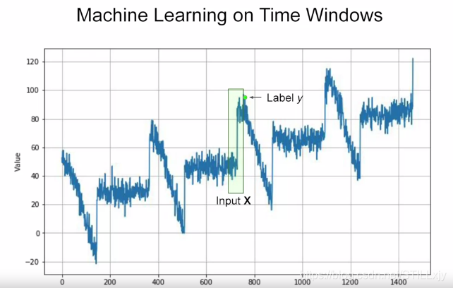
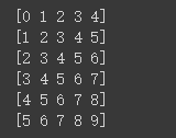
假设上图为某类时间序列问题的历史数据，我们希望“学习”这类数据的规律，预测未来的数据。
为了将数据输入网络，我们需要将数据处理为神经网络需要的 (特征，标签) 类型的数据。

对于时间序列问题，我们引入一个 数据窗口 的概念，如上图绿色框所示。
假设窗口的大小（超参数）为：20， 则表示我们将过去20天的数据作为“特征”数据， 如而将当前的数据作为**“标签”**数据。
遍历所以已知历史数据，我们就可以得到我们所需的数据集。

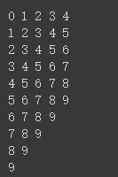
小栗子: 我们以[0,1,2,…,9]的列表（简单序列数据）为例子，使用以上处理方法获得我们所需的数据集
1：导入所需包，确保TensorFlow版本为2.0

!pip install tf-nightly-2.0-preview

import tensorflow as tf
import numpy as np
import matplotlib.pyplot as plt
print(tf.__version__)

2：生成简单的序列数据[0,1,…,9]

dataset = tf.data.Dataset.range(10)
for val in dataset:
   print(val.numpy())

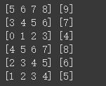
3:获得窗口数据，窗口大小为5（实际为4，最后一个为标签数据）

dataset = tf.data.Dataset.range(10)
dataset = dataset.window(5, shift=1)
for window_dataset in dataset:
  for val in window_dataset:
    print(val.numpy(), end=" ")
  print()

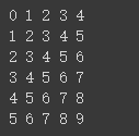
4：将后面不完整的数据去掉，设置 drop_remainder=True

dataset = tf.data.Dataset.range(10)
dataset = dataset.window(5, shift=1, drop_remainder=True)
for window_dataset in dataset:
  for val in window_dataset:
    print(val.numpy(), end=" ")
  print()

5：将数据转换为numpy 列表

dataset = tf.data.Dataset.range(10)
dataset = dataset.window(5, shift=1, drop_remainder=True)
dataset = dataset.flat_map(lambda window: window.batch(5))
for window in dataset:
  print(window.numpy())

6：随机打散数据，将数据分为 特征数据x 和 标签数据y

dataset = tf.data.Dataset.range(10)
dataset = dataset.window(5, shift=1, drop_remainder=True)
dataset = dataset.flat_map(lambda window: window.batch(5))
dataset = dataset.map(lambda window: (window[:-1], window[-1:]))
dataset = dataset.shuffle(buffer_size=10)
for x,y in dataset:
  print(x.numpy(), y.numpy())

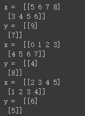
7: 设置数据批量，每两个数据为一批次

dataset = tf.data.Dataset.range(10)
dataset = dataset.window(5, shift=1, drop_remainder=True)
dataset = dataset.flat_map(lambda window: window.batch(5))
dataset = dataset.map(lambda window: (window[:-1], window[-1:]))
dataset = dataset.shuffle(buffer_size=10)
dataset = dataset.batch(2).prefetch(1)
for x,y in dataset:
  print("x = ", x.numpy())
  print("y = ", y.numpy())

将上述实现方法中可变的参数提出，实现相应的从 序列数据 转换为 网络数据集的函数：
参数说明： 序列数据，窗口大小，批次大小，随机缓存大小
输出： (特征， 标签)

def windowed_dataset(series, window_size, batch_size, shuffle_buffer):
  dataset = tf.data.Dataset.from_tensor_slices(series)
  dataset = dataset.window(window_size + 1, shift=1, drop_remainder=True)
  dataset = dataset.flat_map(lambda window: window.batch(window_size + 1))
  dataset = dataset.shuffle(shuffle_buffer).map(lambda window: (window[:-1], window[-1]))
  dataset = dataset.batch(batch_size).prefetch(1)
  return dataset

---

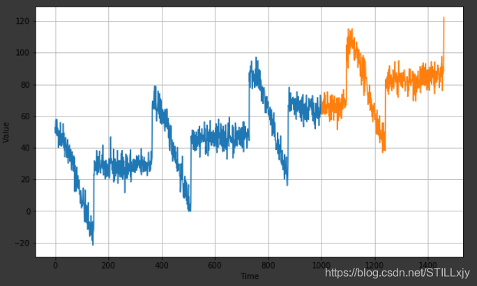
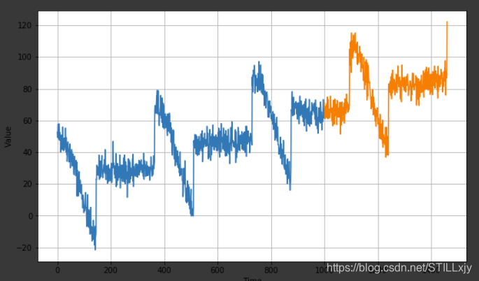
在一个较为复杂的数据上使用神经网络模型进行预测.
如下图所示，蓝色为训练数据， 橙色为验证数据

1：生成上述数据，对于下面的一些函数，仅仅数为了生成上述图片中的数据，可以不必深究

!pip install tf-nightly-2.0-preview

import tensorflow as tf
import numpy as np
import matplotlib.pyplot as plt
print(tf.__version__)

def plot_series(time, series, format="-", start=0, end=None):
    plt.plot(time[start:end], series[start:end], format)
    plt.xlabel("Time")
    plt.ylabel("Value")
    plt.grid(True)

def trend(time, slope=0):
    return slope * time

def seasonal_pattern(season_time):
    """Just an arbitrary pattern, you can change it if you wish"""
    return np.where(season_time < 0.4,
                    np.cos(season_time * 2 * np.pi),
                    1 / np.exp(3 * season_time))

def seasonality(time, period, amplitude=1, phase=0):
    """Repeats the same pattern at each period"""
    season_time = ((time + phase) % period) / period
    return amplitude * seasonal_pattern(season_time)

def noise(time, noise_level=1, seed=None):
    rnd = np.random.RandomState(seed)
    return rnd.randn(len(time)) * noise_level

time = np.arange(4 * 365 + 1, dtype="float32")
baseline = 10
series = trend(time, 0.1)  
baseline = 10
amplitude = 40
slope = 0.05
noise_level = 5

# Create the series
series = baseline + trend(time, slope) + seasonality(time, period=365, amplitude=amplitude)
# Update with noise
series += noise(time, noise_level, seed=42)

2：将数据分为 训练集和验证集（其中加入 time[] 是为了画图方便）

split_time = 1000
time_train = time[:split_time]
x_train = series[:split_time]
time_valid = time[split_time:]
x_valid = series[split_time:]

plt.figure(figsize=(10, 6))

plot_series(time_train, x_train)
plot_series(time_valid, x_valid)

3： 转换数据，适合网络训练

window_size = 20
batch_size = 32
shuffle_buffer_size = 1000

def windowed_dataset(series, window_size, batch_size, shuffle_buffer):
  dataset = tf.data.Dataset.from_tensor_slices(series)
  dataset = dataset.window(window_size + 1, shift=1, drop_remainder=True)
  dataset = dataset.flat_map(lambda window: window.batch(window_size + 1))
  dataset = dataset.shuffle(shuffle_buffer).map(lambda window: (window[:-1], window[-1]))
  dataset = dataset.batch(batch_size).prefetch(1)
  return dataset

dataset = windowed_dataset(x_train, window_size, batch_size, shuffle_buffer_size)
print(dataset)

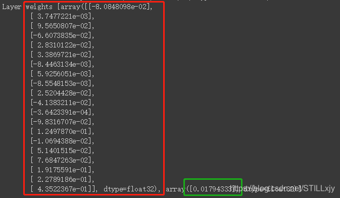
4：定义单层，但神经元网络模型，训练，并数据网络最终参数。红色为W，绿色为b

l0 = tf.keras.layers.Dense(1, input_shape=[window_size])
model = tf.keras.models.Sequential([l0])


model.compile(loss="mse", optimizer=tf.keras.optimizers.SGD(lr=1e-6, momentum=0.9))
model.fit(dataset,epochs=100,verbose=0)

print("Layer weights {}".format(l0.get_weights()))

5: 验证，蓝色为真实数据，橙色为预测数据

forecast = []

for time in range(len(series) - window_size):
  forecast.append(model.predict(series[time:time + window_size][np.newaxis]))

forecast = forecast[split_time-window_size:]
results = np.array(forecast)[:, 0, 0]


plt.figure(figsize=(10, 6))

plot_series(time_valid, x_valid)
plot_series(time_valid, results)

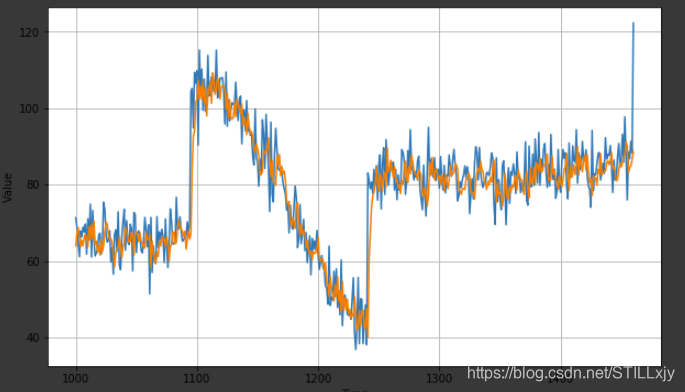
6： 输出mae

tf.keras.metrics.mean_absolute_error(x_valid, results).numpy()