


✅博主简介:热爱科研的Matlab仿真开发者,修心和技术同步精进,Matlab项目合作可私信。
🍎个人主页:海神之光
🏆代码获取方式:
海神之光Matlab王者学习之路—代码获取方式
⛳️座右铭:行百里者,半于九十。
更多Matlab仿真内容点击👇
Matlab图像处理(进阶版)
路径规划(Matlab)
神经网络预测与分类(Matlab)
优化求解(Matlab)
语音处理(Matlab)
信号处理(Matlab)
车间调度(Matlab)
⛄一、A_star算法简介
1 A Star算法及其应用现状
进行搜索任务时提取的有助于简化搜索过程的信息被称为启发信息.启发信息经过文字提炼和公式化后转变为启发函数.启发函数可以表示自起始顶点至目标顶点间的估算距离, 也可以表示自起始顶点至目标顶点间的估算时间等.描述不同的情境、解决不同的问题所采用的启发函数各不相同.我们默认将启发函数命名为H (n) .以启发函数为策略支持的搜索方式我们称之为启发型搜索算法.在救援机器人的路径规划中, A Star算法能结合搜索任务中的环境情况, 缩小搜索范围, 提高搜索效率, 使搜索过程更具方向性、智能性, 所以A Star算法能较好地应用于机器人路径规划相关领域.
2 A Star算法流程
承接2.1节, A Star算法的启发函数是用来估算起始点到目标点的距离, 从而缩小搜索范围, 提高搜索效率.A Star算法的数学公式为:F (n) =G (n) +H (n) , 其中F (n) 是从起始点经由节点n到目标点的估计函数, G (n) 表示从起点移动到方格n的实际移动代价, H (n) 表示从方格n移动到目标点的估算移动代价.
如图2所示, 将要搜寻的区域划分成了正方形的格子, 每个格子的状态分为可通过(walkable) 和不可通过 (unwalkable) .取每个可通过方块的代价值为1, 且可以沿对角移动 (估值不考虑对角移动) .其搜索路径流程如下:

图2 A Star算法路径规划
Step1:定义名为open和closed的两个列表;open列表用于存放所有被考虑来寻找路径的方块, closed列表用于存放不会再考虑的方块;
Step2:A为起点, B为目标点, 从起点A开始, 并将起点A放入open列表中, closed列表初始化为空;
Step3:查看与A相邻的方格n (n称为A的子点, A称为n的父点) , 可通过的方格加入到open列表中, 计算它们的F, G和H值.将A从open移除加入到closed列表中;
Step4:判断open列表是否为空, 如果是, 表示搜索失败, 如果不是, 执行下一步骤;
Step5:将n从open列表移除加入到closed列表中, 判断n是否为目标顶点B, 如果是, 表示搜索成功, 算法运行结束;
Step6:如果不是, 则扩展搜索n的子顶点:
a.如果子顶点是不可通过或在close列表中, 忽略它.
b.子顶点如果不在open列表中, 则加入open列表, 并且把当前方格设置为它的父亲, 记录该方格的F, G和H值.
Step7:跳转到步骤Step4;
Step8:循环结束, 保存路径.从终点开始, 每个方格沿着父节点移动直至起点, 即是最优路径.A Star算法流程图如图3所示.
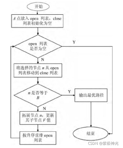
图3 A Star算法流程
⛄二、部分源代码
function varargout = astar_jw(varargin)
if nargin == 0 % Test case, use testCase=2 (Maze) by default

    selectedGrid = 2;
    [grid, init, goal] = defineGrid(selectedGrid);

    % Whether or not to display debug info
    printDebugInfo = true;

elseif nargin == 1 % Test case, set testCase to the input

    selectedGrid = varargin{1};
    [grid, init, goal] = defineGrid(selectedGrid);

    % Whether or not to display debug info
    printDebugInfo = true;

elseif nargin == 3 % Function call with inputs

    grid = varargin{1};
    init = varargin{2};
    goal = varargin{3};

    printDebugInfo = false;

end

% Define all possible moves
delta = [[-1  0]
         [ 0 -1]
         [ 1  0]
         [ 0  1]];

% Add g & f terms to init if necessary
if length(init)==2
    init(3) = 0;    % g
    init(4) = inf;  % f
end

% Perform search
[path, directions] = search(grid, init, goal, delta, printDebugInfo);

if nargout==1
    varargout{1} = path;
elseif nargout==2
    varargout{1} = path;
    varargout{2} = directions;
end
end
function [path, directions] = search(grid, init, goal, delta, printDebugInfo)
% This function implements the A* algorithm
% Initialize the open, closed and path lists
open = []; closed = []; path = [];
open = addRow(open, init);

% Initialize directions list
directions = [];

% Initialize expansion timing grid
expanded = -1 * ones(size(grid));
expanded(open(1), open(2)) = 0;

% Compute the heuristic measurement, h
h = computeHeuristic(grid, goal, 'euclidean');

% Open window for graphical debug display if desired
if printDebugInfo; fig = figure; end

% Keep searching through the grid until the goal is found
goalFound = false;
while size(open,1)>0 && ~goalFound
    [open, closed, expanded] = expand(grid, open, closed, delta, expanded, h);

    % Display debug info if desired
    if printDebugInfo
        displayDebugInfo(grid, init, goal, open, closed, fig);
    end

    goalFound = checkForGoal(closed, goal);
end

% If the goal was found lets get the optimal path
if goalFound
    % We step from the goal to the start location. At each step we
    % select the neighbor with the lowest 'expanded' value and add that
    % neighbor to the path list.
    path = goal;

    % Check to see if the start location is on the path list yet
    [~, indx] = ismember(init(1:2), path(:,1:2), 'rows');
    while ~indx

        % Use our findNeighbors function to find the neighbors of the
        % last location on the path list
        neighbors = findNeighbors(grid, path, size(path,1), delta);

        % Look at the expanded value of all the neighbors, add the one
        % with the lowest expanded value to the path
        expandedVal = expanded(goal(1),goal(2));
        for R = 1:size(neighbors,1)
             neighborExpandedVal = expanded(neighbors(R,1), neighbors(R,2));
             if neighborExpandedVal<expandedVal && neighborExpandedVal>=0
                 chosenNeighbor = R;
                 expandedVal = expanded(neighbors(R,1), neighbors(R,2));
             end
        end
        path(end+1,:) = neighbors(chosenNeighbor,:);

        % Check to see if the start location has been added to the path
        % list yet
        [~, indx] = ismember(init(1:2), path(:,1:2), 'rows');
    end

    % Reorder the list to go from the starting location to the end loc
    path = flipud(path);

    % Compute the directions from the path
    directions = zeros(size(path)-[1 0]);
    for R = 1:size(directions,1)
        directions(R,:) =  path(R+1,:) - path(R,:);
    end

end

% Display results
if printDebugInfo
    home
    if goalFound
        disp(['Goal Found! Distance to goal: ' num2str(closed(goalFound,3))])
        disp(' ')
        disp('Path: ')
        disp(path)

        fig = figure;
        displayPath(grid, path, fig)
    else
        disp('Goal not found!')
    end

    disp(' ')
    disp('Expanded: ')
    disp(expanded)
    disp(' ')
    disp([' Search time to target: ' num2str(expanded(goal(1),goal(2)))])
end
end
function A = deleteRows(A, rows)
% The following way to delete rows was taken from the mathworks website
% that compared multiple ways to do it. The following appeared to be the
% fastest.
index = true(1, size(A,1));
index(rows) = false;
A = A(index, 😃;
end
function A = addRow(A, row)
A(end+1,:) = row;
end
function [open, closed, expanded] = expand(grid, open, closed, delta, expanded, h)
% This function expands the open list by taking the coordinate (row) with
% the smallest f value (path cost) and adds its neighbors to the open list.
% Expand the row with the lowest f
row = find(open(:,4)==min(open(:,4)),1);

% Edit the 'expanded' matrix to note the time in which the current grid
% point was expanded
expanded(open(row,1),open(row,2)) = max(expanded(:))+1;

% Find all the neighbors (potential moves) from the chosen spot
neighbors = findNeighbors(grid, open, row, delta);

% Remove any neighbors that are already on the open or closed lists
neighbors = removeListedNeighbors(neighbors, open, closed);

% Add the neighbors still left to the open list
for R = 1:size(neighbors,1)
    g = open(row,3)+1;
    f = g + h(neighbors(R,1),neighbors(R,2));
    open = addRow(open, [neighbors(R,:) g f] );
end

% Remove the row we just expanded from the open list and add it to the
% closed list
closed(end+1,:) = open(row,:);
open = deleteRows(open, row);
end
function h = computeHeuristic(varargin)
% This function is used to compute the distance heuristic, h. By default
% this function computes the Euclidean distance from each grid space to the
% goal. The calling sequence for this function is as follows:
% h = computeHeuristic(grid, goal[, distanceType])
% where distanceType may be one of the following:
% ‘euclidean’ (default value)
% ‘city-block’
% ‘empty’ (returns all zeros for heuristic function)
grid = varargin{1};
goal = varargin{2};
if nargin==3
distanceType = varargin{3};
else
distanceType = ‘euclidean’;
end
[m n] = size(grid);
[x y] = meshgrid(1:n,1:m);
if strcmp(distanceType, ‘euclidean’)
h = sqrt((x-goal(2)).^2 + (y-goal(1)).^2);
elseif strcmp(distanceType, ‘city-block’)
h = abs(x-goal(2)) + abs(y-goal(1));
elseif strcmp(distanceType, ‘empty’)
h = zeros(m,n);
else
warning(‘Unknown distanceType for determining heuristic, h!’)
h = [];
end
end
function neighbors = findNeighbors(grid, open, row, delta)
% This function takes the desired row in the open list to expand and finds
% all potential neighbors (neighbors reachable through legal moves, as
% defined in the delta list).
% Find the borders to the grid
borders = size(grid);
borders = [1 borders(2) 1 borders(1)]; % [xMin xMax yMin yMax]

% Initialize the current location and neighbors list
cenSq = open(row,1:2);
neighbors = [];

% Go through all the possible moves (given in the 'delta' matrix) and
% add moves not on the closed list
for R = 1:size(delta,1)
    potMove = cenSq + delta(R,:);

    if potMove(1)>=borders(3) && potMove(1)<=borders(4) ...
            && potMove(2)>=borders(1) && potMove(2)<=borders(2)
        if grid(potMove(1), potMove(2))==0
            neighbors(end+1,:) = potMove;
        end
    end
end
end
function neighbors = removeListedNeighbors(neighbors, open, closed)
% This function removes any neighbors that are on the open or closed lists
% Check to make sure there's anything even on the closed list
if size(closed,1)==0
    return
end

% Find any neighbors that are on the open or closed lists
rowsToRemove = [];
for R = 1:size(neighbors)
    % Check to see if the neighbor is on the open list
    [~, indx] = ismember(neighbors(R,:),open(:,1:2),'rows');
    if indx>0
        rowsToRemove(end+1) = R;
    else
        % If the neighbor isn't on the open list, check to make sure it
        % also isn't on the closed list
        [~, indx] = ismember(neighbors(R,:),closed(:,1:2),'rows');
        if indx>0
            rowsToRemove(end+1) = R;
        end
    end
end

% Remove neighbors that were on either the open or closed lists
if numel(rowsToRemove>0)
    neighbors = deleteRows(neighbors, rowsToRemove);
end
end
function goalRow = checkForGoal(closed, goal)
% This function looks for the final goal destination on the closed list.
% Note, you could check the open list instead (and find the goal faster);
% however, we want to have a chance to expand the goal location itself, so
% we wait until it is on the closed list.
[~, goalRow] = ismember(goal, closed(:,1:2), ‘rows’);
end
function displayDebugInfo(grid, init, goal, open, closed, h)
% Display the open and closed lists in the command window, and display an
% image of the current search of the grid.
home
disp('Open: ‘)
disp(open)
disp(’ ')
disp('Closed: ')
disp(closed)
displaySearchStatus(grid, init, goal, open, closed, h)
pause(0.05)
end
function displaySearchStatus(grid, init, goal, open, closed, h)
% This function displays a graphical grid and search status to make
% visualization easier.
grid = double(~grid);
grid(init(1),init(2)) = 0.66;
grid(goal(1),goal(2)) = 0.33;
figure(h)
imagesc(grid); colormap(gray); axis square; axis off; hold on

plot(open(:,2),   open(:,1),   'go', 'LineWidth', 2)
plot(closed(:,2), closed(:,1), 'ro', 'LineWidth', 2)

hold off
end
function displayPath(grid, path, h)
grid = double(~grid);
figure(h)
imagesc(grid); colormap(gray); axis off; hold on
title('Optimal Path', 'FontWeight', 'bold');

plot(path(:,2),  path(:,1),   'co', 'LineWidth', 2)
plot(path(1,2),  path(1,1),   'gs', 'LineWidth', 4)
plot(path(end,2),path(end,1), 'rs', 'LineWidth', 4)
end
⛄三、运行结果


⛄四、matlab版本及参考文献
1 matlab版本
2014a
2 参考文献
[1]钱程,许映秋,谈英姿.A Star算法在RoboCup救援仿真中路径规划的应用[J].指挥与控制学报. 2017,3(03)
3 备注
简介此部分摘自互联网,仅供参考,若侵权,联系删除
🍅 仿真咨询
1 各类智能优化算法改进及应用
生产调度、经济调度、装配线调度、充电优化、车间调度、发车优化、水库调度、三维装箱、物流选址、货位优化、公交排班优化、充电桩布局优化、车间布局优化、集装箱船配载优化、水泵组合优化、解医疗资源分配优化、设施布局优化、可视域基站和无人机选址优化
2 机器学习和深度学习方面
卷积神经网络(CNN)、LSTM、支持向量机(SVM)、最小二乘支持向量机(LSSVM)、极限学习机(ELM)、核极限学习机(KELM)、BP、RBF、宽度学习、DBN、RF、RBF、DELM、XGBOOST、TCN实现风电预测、光伏预测、电池寿命预测、辐射源识别、交通流预测、负荷预测、股价预测、PM2.5浓度预测、电池健康状态预测、水体光学参数反演、NLOS信号识别、地铁停车精准预测、变压器故障诊断
3 图像处理方面
图像识别、图像分割、图像检测、图像隐藏、图像配准、图像拼接、图像融合、图像增强、图像压缩感知
4 路径规划方面
旅行商问题(TSP)、车辆路径问题(VRP、MVRP、CVRP、VRPTW等)、无人机三维路径规划、无人机协同、无人机编队、机器人路径规划、栅格地图路径规划、多式联运运输问题、车辆协同无人机路径规划、天线线性阵列分布优化、车间布局优化
5 无人机应用方面
无人机路径规划、无人机控制、无人机编队、无人机协同、无人机任务分配
6 无线传感器定位及布局方面
传感器部署优化、通信协议优化、路由优化、目标定位优化、Dv-Hop定位优化、Leach协议优化、WSN覆盖优化、组播优化、RSSI定位优化
7 信号处理方面
信号识别、信号加密、信号去噪、信号增强、雷达信号处理、信号水印嵌入提取、肌电信号、脑电信号、信号配时优化
8 电力系统方面
微电网优化、无功优化、配电网重构、储能配置
9 元胞自动机方面
交通流 人群疏散 病毒扩散 晶体生长
10 雷达方面
卡尔曼滤波跟踪、航迹关联、航迹融合


 768
768


 被折叠的 条评论
为什么被折叠?
被折叠的 条评论
为什么被折叠?
 到【灌水乐园】发言


