PyTorch深度学习实战：经典CNN架构与PyTorch Lightning实践

原创于 2025-11-12 09:11:47 发布 · 562 阅读

11 ·

CC 4.0 BY-SA版权

文章标签：

#深度学习 #pytorch #cnn #PTLightning

PyTorch Lightning实践：Inception、ResNet以及DenseNet

学习目标

通过本课程，学员将深入理解 Inception、ResNet 以及 DenseNet 这三种经典卷积神经网络架构的核心思想、结构特点与实现方式，并能对他们在模型性能、训练优化等方面进行对比分析，同时掌握利用 PyTorch Lightning 框架进行模型训练与评估的方法。

学习内容

1 PyTorch Lightning简介

1.1 准备依赖包及数据集

在本课程中，我们将实现和讨论现代 CNN 架构的变体。在过去的几年中，已经提出了许多不同的架构。其中一些最具影响力的架构，并且至今仍然相关的是以下几种：GoogleNet/Inception 架构（ILSVRC 2014 冠军），ResNet（ILSVRC 2015 冠军），以及 DenseNet（CVPR 2017 最佳论文奖）。这些架构在提出时都是最先进的模型，这些网络的核心思想是当前大多数最先进的架构的基础。因此，详细了解这些架构并学习如何实现它们非常重要。
让我们从导入标准库开始。

%pip install seaborn

## Standard libraries
import os
import numpy as np 
import random
from PIL import Image
from types import SimpleNamespace

## Imports for plotting
import matplotlib.pyplot as plt
%matplotlib inline 
from IPython.display import set_matplotlib_formats
set_matplotlib_formats('svg', 'pdf') # For export
import matplotlib
matplotlib.rcParams['lines.linewidth'] = 2.0
import seaborn as sns
sns.reset_orig()

## PyTorch
import torch
import torch.nn as nn
import torch.utils.data as data
import torch.optim as optim
# Torchvision
import torchvision
from torchvision.datasets import CIFAR10
from torchvision import transforms

我们将使用set_seed函数，以及路径变量DATASET_PATH和CHECKPOINT_PATH。如有必要，请调整路径。（下列GPU和MPS二选一即可）：

GPU用户

# 数据集下载/应下载的文件夹路径（例如CIFAR10）
DATASET_PATH = "./cifar_data"
# 保存预训练模型的文件夹路径
CHECKPOINT_PATH = "./saved_models/tutorial5"

# 设置种子的函数
def set_seed(seed):
    random.seed(seed)
    np.random.seed(seed)
    torch.manual_seed(seed)
    if torch.cuda.is_available():
        torch.cuda.manual_seed(seed)
        torch.cuda.manual_seed_all(seed)
set_seed(42)

# 确保所有操作在 GPU 上（如果使用）都是确定性的，以便可重复性
torch.backends.cudnn.deterministic = True
torch.backends.cudnn.benchmark = False

# 优先尝试使用NPU (昇腾)
if hasattr(torch, 'npu') and torch.npu.is_available():  # 检查NPU可用性
    device = torch.device("npu:0")  # 使用第0张NPU卡
else:
    device = torch.device("cpu")  # 降级使用CPU

MPS用户

# 数据集下载/应下载的文件夹路径（例如CIFAR10）
DATASET_PATH = "./cifar_data"
# 保存预训练模型的文件夹路径
CHECKPOINT_PATH = "./saved_models/tutorial5"

# 设置种子的函数
def set_seed(seed):
    random.seed(seed)
    np.random.seed(seed)
    torch.manual_seed(seed)
    # 增加MPS的种子设置（确保MPS随机数可复现）
    if torch.backends.mps.is_available():
        torch.mps.manual_seed(seed)
    elif torch.cuda.is_available():
        torch.cuda.manual_seed(seed)
        torch.cuda.manual_seed_all(seed)

set_seed(42)

# 设备选择逻辑：优先MPS，其次CUDA，最后CPU
if torch.backends.mps.is_available():
    device = torch.device("mps")
    print("Using MPS device")
else:
    device = torch.device("cpu")
    print("Using CPU device")

我们还有预训练模型和 Tensorboards（稍后会详细介绍）用于本课程，请在下面下载它们。

#获取多个模型的预训练权重文件等
!wget https://model-community-picture.obs.cn-north-4.myhuaweicloud.com/ascend-zone/notebook_models/1b54f4a045a511f0b16dfa163edcddae/models.zip
!unzip models.zip

在本课程中，我们将使用 CIFAR10 数据集训练和评估模型。这使学员可以将此处获得的结果与学员在第一个作业中实现的模型进行比较。因此，作为第一步，我们将计算 CIFAR 数据集的均值和标准差：

#获取cifar10数据集
!wget https://model-community-picture.obs.cn-north-4.myhuaweicloud.com/ascend-zone/notebook_datasets/1b54f4a045a511f0b16dfa163edcddae/cifar_dataset.zip
!unzip cifar_dataset.zip

train_dataset = CIFAR10(root=DATASET_PATH, train=True, download=False)
DATA_MEANS = (train_dataset.data / 255.0).mean(axis=(0,1,2))
DATA_STD = (train_dataset.data / 255.0).std(axis=(0,1,2))
print("Data mean", DATA_MEANS)
print("Data std", DATA_STD)

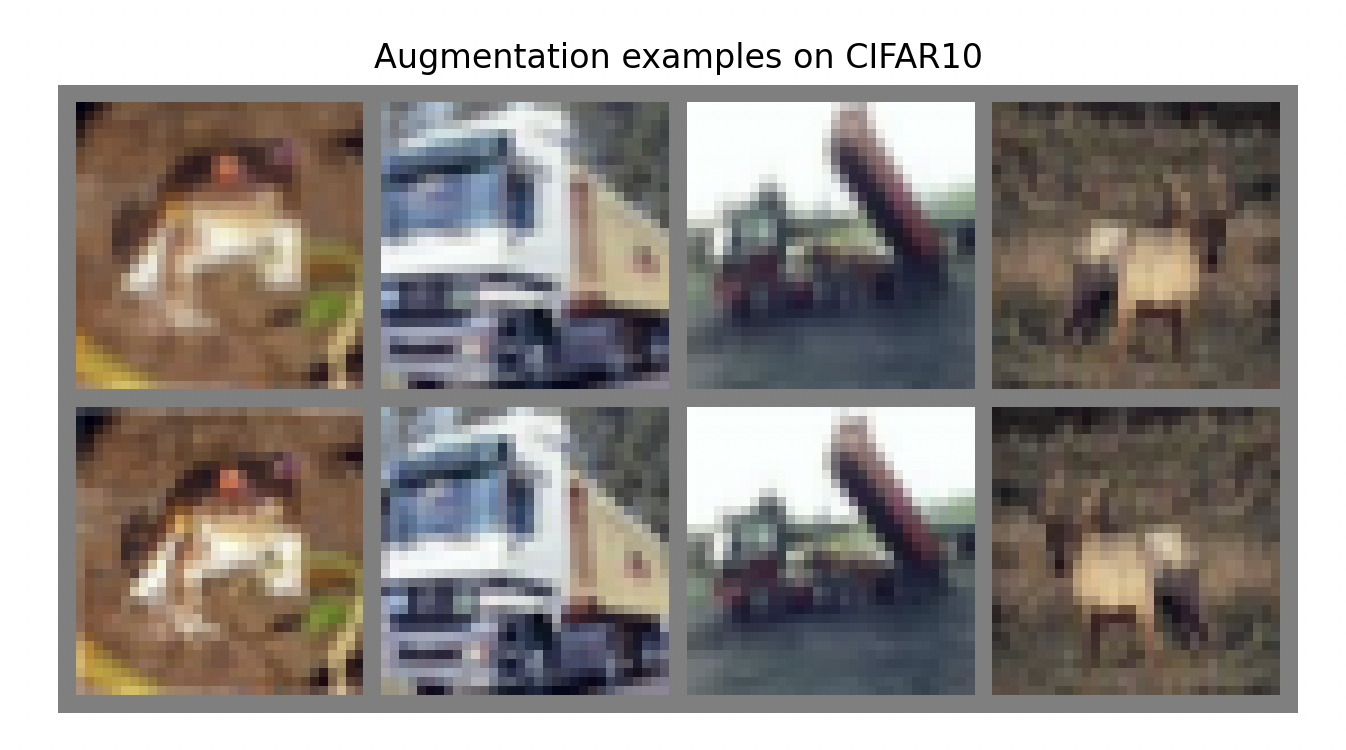
我们将使用这些信息来定义一个transforms.Normalize模块，该模块将相应地规范化我们的数据。此外，我们将在训练期间使用数据增强。这减少了过拟合的风险，并有助于CNN更好地泛化。具体来说，我们将应用两种随机增强。

首先，我们将以50%的概率水平翻转每张图像（transforms.RandomHorizontalFlip）。当翻转图像时，对象类别通常不会改变，我们也不期望任何图像信息依赖于水平方向。然而，如果我们试图检测图像中的数字或字母，情况就会有所不同，因为这些具有特定的方向性。

我们使用的第二种增强称为transforms.RandomResizedCrop。这种变换在一个小范围内裁剪图像，最终改变纵横比，然后将其缩放回原始大小。因此，实际的像素值会发生变化，而图像的内容或整体语义保持不变。

我们将随机将训练数据集分为训练集和验证集。验证集将用于确定提前停止。在完成训练后，我们将在CIFAR测试集上测试模型。

test_transform = transforms.Compose([transforms.ToTensor(),
                                     transforms.Normalize(DATA_MEANS, DATA_STD)
                                     ])
# For training, we add some augmentation. Networks are too powerful and would overfit.
train_transform = transforms.Compose([transforms.RandomHorizontalFlip(),
                                      transforms.RandomResizedCrop((32,32), scale=(0.8,1.0), ratio=(0.9,1.1)),
                                      transforms.ToTensor(),
                                      transforms.Normalize(DATA_MEANS, DATA_STD)
                                     ])
# Loading the training dataset. We need to split it into a training and validation part
# We need to do a little trick because the validation set should not use the augmentation.
train_dataset = CIFAR10(root=DATASET_PATH, train=True, transform=train_transform, download=True)
val_dataset = CIFAR10(root=DATASET_PATH, train=True, transform=test_transform, download=True)
set_seed(42)
train_set, _ = torch.utils.data.random_split(train_dataset, [45000, 5000])
set_seed(42)
_, val_set = torch.utils.data.random_split(val_dataset, [45000, 5000])

# Loading the test set
test_set = CIFAR10(root=DATASET_PATH, train=False, transform=test_transform, download=True)

# We define a set of data loaders that we can use for various purposes later.
train_loader = data.DataLoader(train_set, batch_size=128, shuffle=True, drop_last=True, pin_memory=True, num_workers=4)
val_loader = data.DataLoader(val_set, batch_size=128, shuffle=False, drop_last=False, num_workers=4)
test_loader = data.DataLoader(test_set, batch_size=128, shuffle=False, drop_last=False, num_workers=4)

为了验证我们的归一化是否有效，我们可以打印出单个批次的均值和标准差。每个通道的均值应该接近 0，标准差应该接近 1：

imgs, _ = next(iter(train_loader))
print("Batch mean", imgs.mean(dim=[0,2,3]))
print("Batch std", imgs.std(dim=[0,2,3]))

最后，让我们从训练集中可视化一些图像，并查看它们在随机数据增强后的样子：

NUM_IMAGES = 4
images = [train_dataset[idx][0] for idx in range(NUM_IMAGES)]
orig_images = [Image.fromarray(train_dataset.data[idx]) for idx in range(NUM_IMAGES)]
orig_images = [test_transform(img) for img in orig_images]

img_grid = torchvision.utils.make_grid(torch.stack(images + orig_images, dim=0), nrow=4, normalize=True, pad_value=0.5)
img_grid = img_grid.permute(1, 2, 0)

plt.figure(figsize=(8,8))
plt.title("Augmentation examples on CIFAR10")
plt.imshow(img_grid)
plt.axis('off')
plt.show()
plt.close()

在这里插入图片描述

1.2 PyTorch Lightning

PyTorch Lightning 是一个基于 PyTorch 的轻量化框架，它将 PyTorch 代码中的训练、评估和测试等常用逻辑进行了抽象和封装，使得开发者可以更加专注于模型的架构设计和算法实现。PyTorch Lightning 的核心组件包括 LightningModule 和 Trainer。LightningModule 继承自 torch.nn.Module，它将模型的初始化、优化器设置、训练循环、验证循环和测试循环等功能组织在一个类中，使得代码结构更加清晰。Trainer 则负责执行 LightningModule 中定义的训练步骤，并且提供了丰富的功能，如自动日志记录、模型检查点保存、分布式训练支持等。通过使用 PyTorch Lightning，开发者可以在不牺牲 PyTorch 灵活性的前提下，大大减少代码的冗余，提高开发效率。

在本notebook中，我们将使用库 PyTorch Lightning。PyTorch Lightning 是一个框架，它简化了在 PyTorch 中训练、评估和测试模型所需的代码。它还处理将日志记录到 TensorBoard，这是一个用于机器学习实验的可视化工具包，并自动保存模型检查点，同时将我们的代码开销降到最低。这对我们非常有帮助，因为我们希望专注于实现不同的模型架构，并花费较少的时间在其他代码开销上。请注意，在编写/教学时，该框架已发布为版本 1.8。未来版本可能会稍微更改接口，因此可能无法与代码完美兼容(我们将尽量保持其最新)。首先，我们导入库：

%pip install --quiet pytorch-lightning>=1.5

# PyTorch Lightning
import pytorch_lightning as pl

PyTorch Lightning 包含许多有用的函数，例如用于设置种子的函数：

# Setting the seed
pl.seed_everything(42)

因此，在未来，我们不再需要定义自己的 set_seed 函数了。
在 PyTorch Lightning 中，我们定义 pl.LightningModule（继承自 torch.nn.Module），将代码组织成 5 个主要部分：

初始化 (__init__)，在这里我们创建所有必要的参数/模型
优化器 (configure_optimizers)，在这里我们创建优化器、学习率调度器等。
训练循环 (training_step)，在这里我们只需要定义单个批次的损失计算（优化器的 zero_grad()、loss.backward() 和 optimizer.step() 循环，以及任何日志记录/保存操作，都在后台完成）
验证循环 (validation_step)，与训练类似，我们只需要定义每一步应该发生什么
测试循环 (test_step)，与验证相同，只是针对测试集。
因此，我们并没有抽象 PyTorch 代码，而是组织代码并定义一些常用的默认操作。如果您需要在训练/验证/测试循环中更改其他内容，有许多可能的函数可以覆盖。

现在我们可以看看一个用于训练 CNN 的 Lightning Module 的示例：

class CIFARModule(pl.LightningModule):

    def __init__(self, model_name, model_hparams, optimizer_name, optimizer_hparams):
        """
        Inputs:
            model_name - Name of the model/CNN to run. Used for creating the model (see function below)
            model_hparams - Hyperparameters for the model, as dictionary.
            optimizer_name - Name of the optimizer to use. Currently supported: Adam, SGD
            optimizer_hparams - Hyperparameters for the optimizer, as dictionary. This includes learning rate, weight decay, etc.
        """
        super().__init__()
        # Exports the hyperparameters to a YAML file, and create "self.hparams" namespace
        self.save_hyperparameters()
        # Create model
        self.model = create_model(model_name, model_hparams)
        # Create loss module
        self.loss_module = nn.CrossEntropyLoss()
        # Example input for visualizing the graph in Tensorboard
        self.example_input_array = torch.zeros((1, 3, 32, 32), dtype=torch.float32)

    def forward(self, imgs):
        # Forward function that is run when visualizing the graph
        return self.model(imgs)

    def configure_optimizers(self):
        # We will support Adam or SGD as optimizers.
        if self.hparams.optimizer_name == "Adam":
            # AdamW is Adam with a correct implementation of weight decay (see here for details: https://arxiv.org/pdf/1711.05101.pdf)
            optimizer = optim.AdamW(
                self.parameters(), **self.hparams.optimizer_hparams)
        elif self.hparams.optimizer_name == "SGD":
            optimizer = optim.SGD(self.parameters(), **self.hparams.optimizer_hparams)
        else:
            assert False, f"Unknown optimizer: \"{self.hparams.optimizer_name}\""

        # We will reduce the learning rate by 0.1 after 100 and 150 epochs
        scheduler = optim.lr_scheduler.MultiStepLR(
            optimizer, milestones=[100, 150], gamma=0.1)
        return [optimizer], [scheduler]

    def training_step(self, batch, batch_idx):
        # "batch" is the output of the training data loader.
        imgs, labels = batch
        preds = self.model(imgs)
        loss = self.loss_module(preds, labels)
        acc = (preds.argmax(dim=-1) == labels).float().mean()

        # Logs the accuracy per epoch to tensorboard (weighted average over batches)
        self.log('train_acc', acc, on_step=False, on_epoch=True)
        self.log('train_loss', loss)
        return loss  # Return tensor to call ".backward" on

    def validation_step(self, batch, batch_idx):
        imgs, labels = batch
        preds = self.model(imgs).argmax(dim=-1)
        acc = (labels == preds).float().mean()
        # By default logs it per epoch (weighted average over batches)
        self.log('val_acc', acc)

    def test_step(self, batch, batch_idx):
        imgs, labels = batch
        preds = self.model(imgs).argmax(dim=-1)
        acc = (labels == preds).float().mean()
        # By default logs it per epoch (weighted average over batches), and returns it afterwards
        self.log('test_acc', acc)

PyTorch Lightning 的另一个重要部分是回调函数的概念。回调函数是包含 Lightning 模块非必要逻辑的独立函数。它们通常在完成一个训练周期后被调用，但也可以影响训练循环的其他部分。例如，我们将使用以下两个预定义的回调函数：LearningRateMonitor 和 ModelCheckpoint。学习率监视器将当前学习率添加到我们的 TensorBoard 中，这有助于验证我们的学习率调度器是否正常工作。模型检查点回调函数允许学员自定义检查点的保存方式。例如，保存多少个检查点，何时保存，关注哪个指标等。我们在下面导入它们：

# Callbacks 
from pytorch_lightning.callbacks import LearningRateMonitor, ModelCheckpoint

为了允许使用相同的 Lightning 模块运行多个不同的模型，我们在下面定义了一个函数，该函数将模型名称映射到模型类。在这个阶段，字典 model_dict 是空的，但我们将通过我们的新模型在整个notebook中填充它。

model_dict = {}

def create_model(model_name, model_hparams):
    if model_name in model_dict:
        return model_dict[model_name](**model_hparams)
    else:
        assert False, f"Unknown model name \"{model_name}\". Available models are: {str(model_dict.keys())}"

同样，为了将激活函数作为我们模型的另一个超参数，我们在下面定义了一个“名称到函数”的字典：

act_fn_by_name = {
    "tanh": nn.Tanh,
    "relu": nn.ReLU,
    "leakyrelu": nn.LeakyReLU,
    "gelu": nn.GELU
}

如果我们直接将类或对象作为参数传递给 Lightning 模块，我们就无法利用 PyTorch Lightning 自动保存和加载超参数的功能。

除了 Lightning 模块，PyTorch Lightning 中第二重要的模块是 Trainer。Trainer 负责执行 Lightning 模块中定义的训练步骤，并完成框架。与 Lightning 模块类似，您可以覆盖任何不想自动化的关键部分，但默认设置通常是最佳实践。我们在下面使用的最重要的函数是：

trainer.fit：接受一个 Lightning 模块、一个训练数据集和一个（可选的）验证数据集作为输入。此函数在训练数据集上训练给定的模块，并偶尔进行验证（默认每轮一次，可以更改）。
trainer.test：接受一个模型和一个我们希望测试的数据集作为输入。它返回数据集上的测试指标。

在训练和测试时，我们无需担心将模型设置为评估模式（model.eval()）等问题，因为这些都已自动完成。请参阅下面我们如何为模型定义训练函数：

def train_model(model_name, save_name=None, **kwargs):
    """
    Inputs:
        model_name - Name of the model you want to run. Is used to look up the class in "model_dict"
        save_name (optional) - If specified, this name will be used for creating the checkpoint and logging directory.
    """
    if save_name is None:
        save_name = model_name
        
    # Create a PyTorch Lightning trainer with the generation callback
    trainer = pl.Trainer(default_root_dir=os.path.join(CHECKPOINT_PATH, save_name),                          # Where to save models
                         accelerator="gpu" if str(device).startswith("cuda") else "cpu",                     # We run on a GPU (if possible)
                         devices=1,                                                                          # How many GPUs/CPUs we want to use (1 is enough for the notebooks)
                         max_epochs=180,                                                                     # How many epochs to train for if no patience is set
                         callbacks=[ModelCheckpoint(save_weights_only=True, mode="max", monitor="val_acc"),  # Save the best checkpoint based on the maximum val_acc recorded. Saves only weights and not optimizer
                                    LearningRateMonitor("epoch")],                                           # Log learning rate every epoch
                         enable_progress_bar=True)                                                           # Set to False if you do not want a progress bar
    trainer.logger._log_graph = True         # If True, we plot the computation graph in tensorboard
    trainer.logger._default_hp_metric = None # Optional logging argument that we don't need
    
    # Check whether pretrained model exists. If yes, load it and skip training
    pretrained_filename = os.path.join(CHECKPOINT_PATH, save_name + ".ckpt")
    if os.path.isfile(pretrained_filename):
        print(f"Found pretrained model at {pretrained_filename}, loading...")
        model = CIFARModule.load_from_checkpoint(pretrained_filename) # Automatically loads the model with the saved hyperparameters
    else:
        pl.seed_everything(42) # To be reproducable
        model = CIFARModule(model_name=model_name, **kwargs)
        trainer.fit(model, train_loader, val_loader)
        model = CIFARModule.load_from_checkpoint(trainer.checkpoint_callback.best_model_path) # Load best checkpoint after training
        
    # Test best model on validation and test set
    val_result = trainer.test(model, val_loader, verbose=False)
    test_result = trainer.test(model, test_loader, verbose=False)
    result = {"test": test_result[0]["test_acc"], "val": val_result[0]["test_acc"]}
    
    return model, result

2 PyTorch Lightning实战经典CNN模型

2.1 基于Inception架构

2.1.1 Inception Block

2014年提出的GoogleNet因使用了Inception模块而赢得了ImageNet挑战赛。总的来说，我们将在本课程中主要关注Inception的概念，而不是GoogleNet的具体内容，因为基于Inception，已经有很多后续作品(Inception-v2、Inception-v3、Inception-v4、Inception-ResNet、…后续的工作主要集中在提高效率和使能非常深入的Inception网络。但是，对于一个基本的理解，看看原始的Inception块就足够了。

Inception块在同一个feature map上分别应用4个卷积块：1x1、3x3和5x5卷积，以及最大池操作。这使得网络可以使用不同的感受野查看相同的数据。当然，只学习5x5卷积理论上会更强大。然而，这不仅计算量和内存量更大，而且容易发生过拟合。

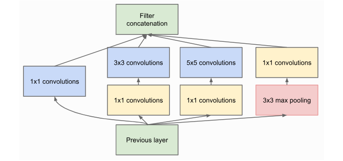
图1：Inception整体起始块

在 3x3 和 5x5 卷积之前添加的 1x1 卷积用于降维。这尤其重要，因为所有分支的特征图在之后会被合并，我们不希望特征大小爆炸。由于 5x5 卷积比 1x1 卷积昂贵 25 倍，我们可以通过在大卷积之前降低维度来节省大量计算和参数。

现在我们可以尝试自己实现Inception Block：

class InceptionBlock(nn.Module):
    
    def __init__(self, c_in, c_red : dict, c_out : dict, act_fn):
        """
        Inputs:
            c_in - Number of input feature maps from the previous layers
            c_red - Dictionary with keys "3x3" and "5x5" specifying the output of the dimensionality reducing 1x1 convolutions
            c_out - Dictionary with keys "1x1", "3x3", "5x5", and "max"
            act_fn - Activation class constructor (e.g. nn.ReLU)
        """
        super().__init__()
        
        # 1x1 convolution branch
        self.conv_1x1 = nn.Sequential(
            nn.Conv2d(c_in, c_out["1x1"], kernel_size=1),
            nn.BatchNorm2d(c_out["1x1"]),
            act_fn()
        )
        
        # 3x3 convolution branch
        self.conv_3x3 = nn.Sequential(
            nn.Conv2d(c_in, c_red["3x3"], kernel_size=1),
            nn.BatchNorm2d(c_red["3x3"]),
            act_fn(),
            nn.Conv2d(c_red["3x3"], c_out["3x3"], kernel_size=3, padding=1),
            nn.BatchNorm2d(c_out["3x3"]),
            act_fn()
        )
        
        # 5x5 convolution branch
        self.conv_5x5 = nn.Sequential(
            nn.Conv2d(c_in, c_red["5x5"], kernel_size=1),
            nn.BatchNorm2d(c_red["5x5"]),
            act_fn(),
            nn.Conv2d(c_red["5x5"], c_out["5x5"], kernel_size=5, padding=2),
            nn.BatchNorm2d(c_out["5x5"]),
            act_fn()
        )
        
        # Max-pool branch
        self.max_pool = nn.Sequential(
            nn.MaxPool2d(kernel_size=3, padding=1, stride=1),
            nn.Conv2d(c_in, c_out["max"], kernel_size=1),
            nn.BatchNorm2d(c_out["max"]),
            act_fn()
        )

    def forward(self, x):
        x_1x1 = self.conv_1x1(x)
        x_3x3 = self.conv_3x3(x)
        x_5x5 = self.conv_5x5(x)
        x_max = self.max_pool(x)
        x_out = torch.cat([x_1x1, x_3x3, x_5x5, x_max], dim=1)
        return x_out

GoogleNet 架构由多个 Inception 块堆叠而成，偶尔使用最大池化来减少特征图的高度和宽度。原始的 GoogleNet 是为 ImageNet（224x224 像素）图像大小设计的，拥有近 700 万个参数。由于我们在 CIFAR10 上训练，图像大小为 32x32，因此不需要如此复杂的架构，而是应用了一个简化版本。维度降低和每个滤波器（1x1、3x3、5x5 和最大池化）的输出通道数需要手动指定，如果感兴趣，可以更改。一般直觉是让 3x3 卷积的滤波器数量最多，因为它们足够强大，可以考虑到上下文，同时只需要 5x5 卷积参数的三分之一。

class GoogleNet(nn.Module):

    def __init__(self, num_classes=10, act_fn_name="relu", **kwargs):
        super().__init__()
        self.hparams = SimpleNamespace(num_classes=num_classes,
                                       act_fn_name=act_fn_name,
                                       act_fn=act_fn_by_name[act_fn_name])
        self._create_network()
        self._init_params()

    def _create_network(self):
        # A first convolution on the original image to scale up the channel size
        self.input_net = nn.Sequential(
            nn.Conv2d(3, 64, kernel_size=3, padding=1),
            nn.BatchNorm2d(64),
            self.hparams.act_fn()
        )
        # Stacking inception blocks
        self.inception_blocks = nn.Sequential(
            InceptionBlock(64, c_red={"3x3": 32, "5x5": 16}, c_out={"1x1": 16, "3x3": 32, "5x5": 8, "max": 8}, act_fn=self.hparams.act_fn),
            InceptionBlock(64, c_red={"3x3": 32, "5x5": 16}, c_out={"1x1": 24, "3x3": 48, "5x5": 12, "max": 12}, act_fn=self.hparams.act_fn),
            nn.MaxPool2d(3, stride=2, padding=1),  # 32x32 => 16x16
            InceptionBlock(96, c_red={"3x3": 32, "5x5": 16}, c_out={"1x1": 24, "3x3": 48, "5x5": 12, "max": 12}, act_fn=self.hparams.act_fn),
            InceptionBlock(96, c_red={"3x3": 32, "5x5": 16}, c_out={"1x1": 16, "3x3": 48, "5x5": 16, "max": 16}, act_fn=self.hparams.act_fn),
            InceptionBlock(96, c_red={"3x3": 32, "5x5": 16}, c_out={"1x1": 16, "3x3": 48, "5x5": 16, "max": 16}, act_fn=self.hparams.act_fn),
            InceptionBlock(96, c_red={"3x3": 32, "5x5": 16}, c_out={"1x1": 32, "3x3": 48, "5x5": 24, "max": 24}, act_fn=self.hparams.act_fn),
            nn.MaxPool2d(3, stride=2, padding=1),  # 16x16 => 8x8
            InceptionBlock(128, c_red={"3x3": 48, "5x5": 16}, c_out={"1x1": 32, "3x3": 64, "5x5": 16, "max": 16}, act_fn=self.hparams.act_fn),
            InceptionBlock(128, c_red={"3x3": 48, "5x5": 16}, c_out={"1x1": 32, "3x3": 64, "5x5": 16, "max": 16}, act_fn=self.hparams.act_fn)
        )
        # Mapping to classification output
        self.output_net = nn.Sequential(
            nn.AdaptiveAvgPool2d((1, 1)),
            nn.Flatten(),
            nn.Linear(128, self.hparams.num_classes)
        )

    def _init_params(self):
        # Based on our discussion in Tutorial 4, we should initialize the convolutions according to the activation function
        for m in self.modules():
            if isinstance(m, nn.Conv2d):
                nn.init.kaiming_normal_(
                    m.weight, nonlinearity=self.hparams.act_fn_name)
            elif isinstance(m, nn.BatchNorm2d):
                nn.init.constant_(m.weight, 1)
                nn.init.constant_(m.bias, 0)

    def forward(self, x):
        x = self.input_net(x)
        x = self.inception_blocks(x)
        x = self.output_net(x)
        return x

现在，我们可以将我们的模型集成到我们上面定义的模型字典中：

model_dict["GoogleNet"] = GoogleNet

模型的训练由 PyTorch Lightning 处理，我们只需要定义启动命令。请注意，我们训练了近 200 个 epoch，这在 Snellius 的默认 GPU（NVIDIA A100）上不到一个小时。如果您感兴趣，我们建议您使用保存的模型并训练自己的模型。

googlenet_model, googlenet_results = train_model(model_name="GoogleNet", 
                                                 model_hparams={"num_classes": 10, 
                                                                "act_fn_name": "relu"}, 
                                                 optimizer_name="Adam",
                                                 optimizer_hparams={"lr": 1e-3,
                                                                    "weight_decay": 1e-4})

我们稍后在notebook中比较结果，但我们可以在这里打印它们，以获得初步印象：

print("GoogleNet Results", googlenet_results)

out:
GoogleNet Results {‘test’: 0.8970000147819519, ‘val’: 0.9039999842643738}

2.1.2 Tensorboard日志

PyTorch Lightning的一个不错的额外功能是自动登录到TensorBoard。为了让学员更好地直观地了解TensorBoard可以用于什么，我们可以查看PyTorch Lightning在训练GoogleNet时生成的板。TensorBoard为Jupyter notebook提供了内联功能，我们在这里展示可视化示例：

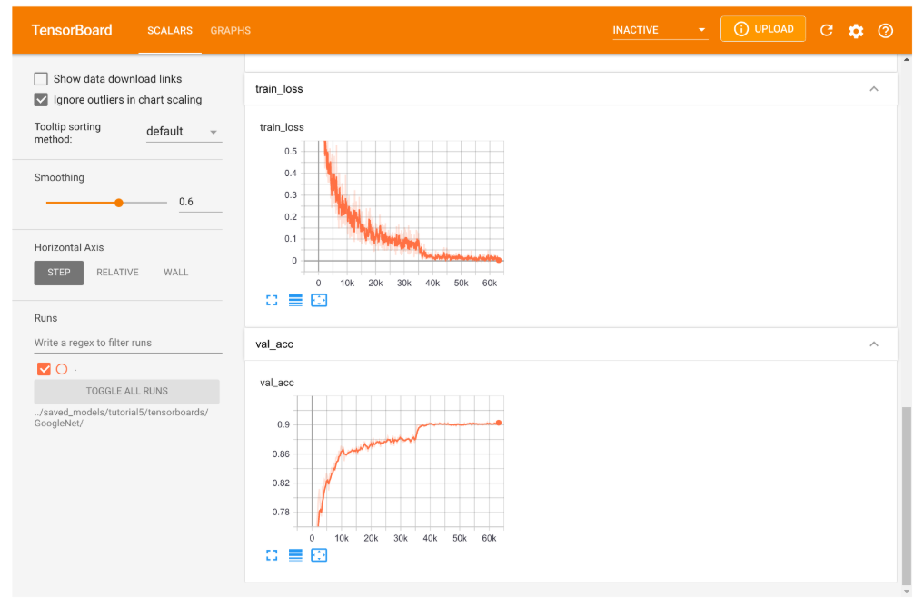
图2：Inception模型训练的TensorBoard可视化展示

TensorBoard 被组织成多个选项卡。主选项卡是标量选项卡，在这里我们可以记录单个数字的发展情况。例如，我们绘制了训练损失、准确率、学习率等。如果我们查看训练或验证准确率，我们可以真正看到使用学习率调度器的影响。降低学习率使我们的模型在训练性能上有了很好的提升。同样，当我们查看训练损失时，我们看到在这个点上有一个突然的下降。然而，与验证集相比，训练集上的高数值表明我们的模型过拟合了，对于如此大的网络来说这是不可避免的。

TensorBoard 中另一个有趣的选项卡是图表选项卡。它向我们展示了从输入到输出的网络架构，按构建块组织。它基本上显示了 CIFARModule 前向步骤中执行的操作。双击一个模块以打开它。请随意从不同的角度探索架构。图表可视化通常可以帮助您验证您的模型实际上正在执行它应该执行的操作，并且您没有在计算图中遗漏任何层。

2.2 ResNet

2.2.1 ResNetBlock

ResNet论文是被引用次数最多的AI论文之一,也是拥有超过1000层的神经网络的基础。尽管其简单，残差连接的思想是非常有效的，因为它支持通过网络稳定的梯度传播。我们不对 $x_{l+1}=F(x_{l}）$ 建模，而是对 $x_{l+1}=x_{l}+F(x_{l})$ 建模，其中 $F$ 是非线性映射（通常是NN模块序列，如卷积、激活函数、和归一化）。如果我们在这样的残差连接上进行反向传播，我们得到：

$\frac{\partial x_{l+1}}{\partial x_{l}} = \mathbf{I} + \frac{\partial F(x_{l})}{\partial x_{l}}$

对单位矩阵的偏向保证了稳定的梯度传播较少受到 $F$ 本身的影响。已经提出了许多ResNet的变体，这些变体主要涉及函数 $F$ ，或应用在和上的操作。在本课程中，我们将介绍其中的两个：原始ResNet块和预激活ResNet块。我们直观地比较了下面的块：

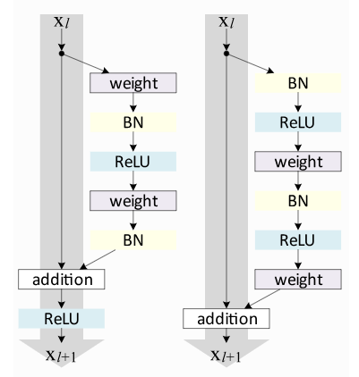
图3：原始ResNet块和预激活ResNet块结构图

原始的ResNet块在跳跃连接之后应用非线性激活函数，通常是ReLU。相反，预激活ResNet块在 $F$ 开始时应用非线性。两者各有利弊。然而，对于非常深的网络，预激活ResNet已经显示出更好的性能，因为梯度流保证具有如上所述计算的单位矩阵，并且不会受到应用于它的任何非线性激活的损害。为了进行比较，在本笔记中，我们将两种ResNet类型实现为浅层网络。

让我们从最初的ResNet块开始。上面的可视化已经显示了 $F$ 中包含了哪些层。我们必须处理的一个特殊情况是，当我们想在宽度和高度方面减少图像尺寸时。基本ResNet块要求 $F(x_{l})$ 与 $x_{l}$ 具有相同的形状。因此，在添加到 $F(x_{l})$ 之前，我们也需要改变 $x_{l}$ 的维数。原始实现使用跨度为2的标识映射，并使用0填充额外的特征维度。然而，更常见的实现是使用stride为2的1x1卷积，因为它允许我们在参数和计算成本上高效地改变特征维度。ResNet块的代码相对简单，如下所示：

class ResNetBlock(nn.Module):

    def __init__(self, c_in, act_fn, subsample=False, c_out=-1):
        """
        Inputs:
            c_in - Number of input features
            act_fn - Activation class constructor (e.g. nn.ReLU)
            subsample - If True, we want to apply a stride inside the block and reduce the output shape by 2 in height and width
            c_out - Number of output features. Note that this is only relevant if subsample is True, as otherwise, c_out = c_in
        """
        super().__init__()
        if not subsample:
            c_out = c_in
            
        # Network representing F
        self.net = nn.Sequential(
            nn.Conv2d(c_in, c_out, kernel_size=3, padding=1, stride=1 if not subsample else 2, bias=False),  # No bias needed as the Batch Norm handles it
            nn.BatchNorm2d(c_out),
            act_fn(),
            nn.Conv2d(c_out, c_out, kernel_size=3, padding=1, bias=False),
            nn.BatchNorm2d(c_out)
        )
        
        # 1x1 convolution with stride 2 means we take the upper left value, and transform it to new output size
        self.downsample = nn.Conv2d(c_in, c_out, kernel_size=1, stride=2) if subsample else None
        self.act_fn = act_fn()

    def forward(self, x):
        z = self.net(x)
        if self.downsample is not None:
            x = self.downsample(x)
        out = z + x
        out = self.act_fn(out)
        return out

我们实现的第二个块是预激活 ResNet 块。为此，我们需要更改 self.net 中的层顺序，并且不对输出应用激活函数。此外，下采样操作必须应用非线性，因为输入 $x_l$ 尚未经过非线性处理。因此，该块如下所示：

class PreActResNetBlock(nn.Module):

    def __init__(self, c_in, act_fn, subsample=False, c_out=-1):
        """
        Inputs:
            c_in - Number of input features
            act_fn - Activation class constructor (e.g. nn.ReLU)
            subsample - If True, we want to apply a stride inside the block and reduce the output shape by 2 in height and width
            c_out - Number of output features. Note that this is only relevant if subsample is True, as otherwise, c_out = c_in
        """
        super().__init__()
        if not subsample:
            c_out = c_in
            
        # Network representing F
        self.net = nn.Sequential(
            nn.BatchNorm2d(c_in),
            act_fn(),
            nn.Conv2d(c_in, c_out, kernel_size=3, padding=1, stride=1 if not subsample else 2, bias=False),
            nn.BatchNorm2d(c_out),
            act_fn(),
            nn.Conv2d(c_out, c_out, kernel_size=3, padding=1, bias=False)
        )
        
        # 1x1 convolution can apply non-linearity as well, but not strictly necessary
        self.downsample = nn.Sequential(
            nn.BatchNorm2d(c_in),
            act_fn(),
            nn.Conv2d(c_in, c_out, kernel_size=1, stride=2, bias=False)
        ) if subsample else None

    def forward(self, x):
        z = self.net(x)
        if self.downsample is not None:
            x = self.downsample(x)
        out = z + x
        return out

与模型选择类似，我们定义一个字典，用于将字符串映射到块类。我们将使用字符串名称作为模型中的超参数值，以在 ResNet 块之间进行选择。请随意实现其他 ResNet 块类型，并将其添加到此处。
ResNet的整体架构由多个ResNet块堆叠而成，其中一些块对输入进行下采样。在讨论整个网络中的ResNet块时，我们通常将它们按相同的输出形状分组。因此，如果我们说ResNet有[3,3,3]块，这意味着我们有3组3个ResNet块，其中第4个和第7个块进行下采样。在CIFAR10上的[3,3,3]块ResNet如下所示。

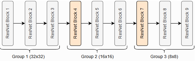
图4：在CIFAR10上的ResNet[3,3,3]块

这三组分别在分辨率 $32\times32$ 、 $16\times16$ 和 $8\times8$ 上操作。橙色块表示具有下采样的ResNet块。许多其他实现也使用相同的符号，例如PyTorch中的torchvision库。因此，我们的代码如下所示：

class ResNet(nn.Module):

    def __init__(self, num_classes=10, num_blocks=[3,3,3], c_hidden=[16,32,64], act_fn_name="relu", block_name="ResNetBlock", **kwargs):
        """
        Inputs: 
            num_classes - Number of classification outputs (10 for CIFAR10)
            num_blocks - List with the number of ResNet blocks to use. The first block of each group uses downsampling, except the first.
            c_hidden - List with the hidden dimensionalities in the different blocks. Usually multiplied by 2 the deeper we go.
            act_fn_name - Name of the activation function to use, looked up in "act_fn_by_name"
            block_name - Name of the ResNet block, looked up in "resnet_blocks_by_name"
        """
        super().__init__()
        assert block_name in resnet_blocks_by_name
        self.hparams = SimpleNamespace(num_classes=num_classes, 
                                       c_hidden=c_hidden, 
                                       num_blocks=num_blocks, 
                                       act_fn_name=act_fn_name,
                                       act_fn=act_fn_by_name[act_fn_name],
                                       block_class=resnet_blocks_by_name[block_name])
        self._create_network()
        self._init_params()

    def _create_network(self):
        c_hidden = self.hparams.c_hidden
        
        # A first convolution on the original image to scale up the channel size
        if self.hparams.block_class == PreActResNetBlock: # => Don't apply non-linearity on output
            self.input_net = nn.Sequential(
                nn.Conv2d(3, c_hidden[0], kernel_size=3, padding=1, bias=False)
            )
        else:
            self.input_net = nn.Sequential(
                nn.Conv2d(3, c_hidden[0], kernel_size=3, padding=1, bias=False),
                nn.BatchNorm2d(c_hidden[0]),
                self.hparams.act_fn()
            )
        
        # Creating the ResNet blocks
        blocks = []
        for block_idx, block_count in enumerate(self.hparams.num_blocks):
            for bc in range(block_count):
                subsample = (bc == 0 and block_idx > 0) # Subsample the first block of each group, except the very first one.
                blocks.append(
                    self.hparams.block_class(c_in=c_hidden[block_idx if not subsample else (block_idx-1)],
                                             act_fn=self.hparams.act_fn,
                                             subsample=subsample,
                                             c_out=c_hidden[block_idx])
                )
        self.blocks = nn.Sequential(*blocks)
        
        # Mapping to classification output
        self.output_net = nn.Sequential(
            nn.AdaptiveAvgPool2d((1,1)),
            nn.Flatten(),
            nn.Linear(c_hidden[-1], self.hparams.num_classes)
        )

    def _init_params(self):
        # Based on our discussion in Tutorial 4, we should initialize the convolutions according to the activation function
        # Fan-out focuses on the gradient distribution, and is commonly used in ResNets
        for m in self.modules():
            if isinstance(m, nn.Conv2d):
                nn.init.kaiming_normal_(m.weight, mode='fan_out', nonlinearity=self.hparams.act_fn_name)
            elif isinstance(m, nn.BatchNorm2d):
                nn.init.constant_(m.weight, 1)
                nn.init.constant_(m.bias, 0)

    def forward(self, x):
        x = self.input_net(x)
        x = self.blocks(x)
        x = self.output_net(x)
        return x

我们还需要将新的ResNet类添加到模型字典中：

model_dict["ResNet"] = ResNet

最后，我们可以训练我们的ResNet模型。与GoogleNet训练的一个不同之处在于，我们明确使用带有动量的SGD作为优化器，而不是Adam。Adam通常会导致在简单的浅层ResNet上准确率稍差。为什么Adam在这种情况下表现更差并不完全清楚，但一个可能的解释与ResNet的损失表面有关。ResNet已被证明比没有跳过连接的网络产生更平滑的损失表面。带有/不带跳过连接的损失表面的可能可视化如下所示：

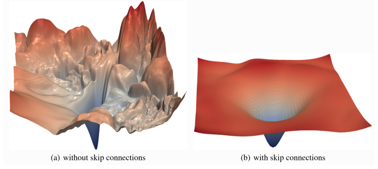
图5：ResNet带有/不带跳过连接的损失表面图

$x$ 和 $y$ 轴显示了参数空间的投影， $z$ 轴显示了不同参数值所达到的损失值。在像右侧那样的平滑表面上，我们可能不需要Adam提供的自适应学习率。相反，Adam可能会陷入局部最优，而SGD可以找到更宽泛的最小值，这些最小值往往具有更好的泛化能力。
然而，要详细回答这个问题，我们需要一个额外的实验，因为这个问题并不容易回答。目前，我们得出结论：对于ResNet架构，将优化器视为一个重要的超参数，并尝试使用Adam和SGD进行训练。让我们使用SGD训练下面的模型：

resnet_model, resnet_results = train_model(model_name="ResNet", 
                                           model_hparams={"num_classes": 10,
                                                          "c_hidden": [16,32,64],
                                                          "num_blocks": [3,3,3],
                                                          "act_fn_name": "relu"}, 
                                           optimizer_name="SGD",
                                           optimizer_hparams={"lr": 0.1,
                                                              "momentum": 0.9,
                                                              "weight_decay": 1e-4})

我们还可以训练预激活的ResNet作为对比：

resnetpreact_model, resnetpreact_results = train_model(model_name="ResNet", 
                                                       model_hparams={"num_classes": 10,
                                                                      "c_hidden": [16,32,64],
                                                                      "num_blocks": [3,3,3],
                                                                      "act_fn_name": "relu",
                                                                      "block_name": "PreActResNetBlock"}, 
                                                       optimizer_name="SGD",
                                                       optimizer_hparams={"lr": 0.1,
                                                                          "momentum": 0.9,
                                                                          "weight_decay": 1e-4},
                                                       save_name="ResNetPreAct")

2.2.2 Tensorboard 日志

与我们的 GoogleNet 模型类似，我们也有一个 ResNet 模型的 TensorBoard 日志。

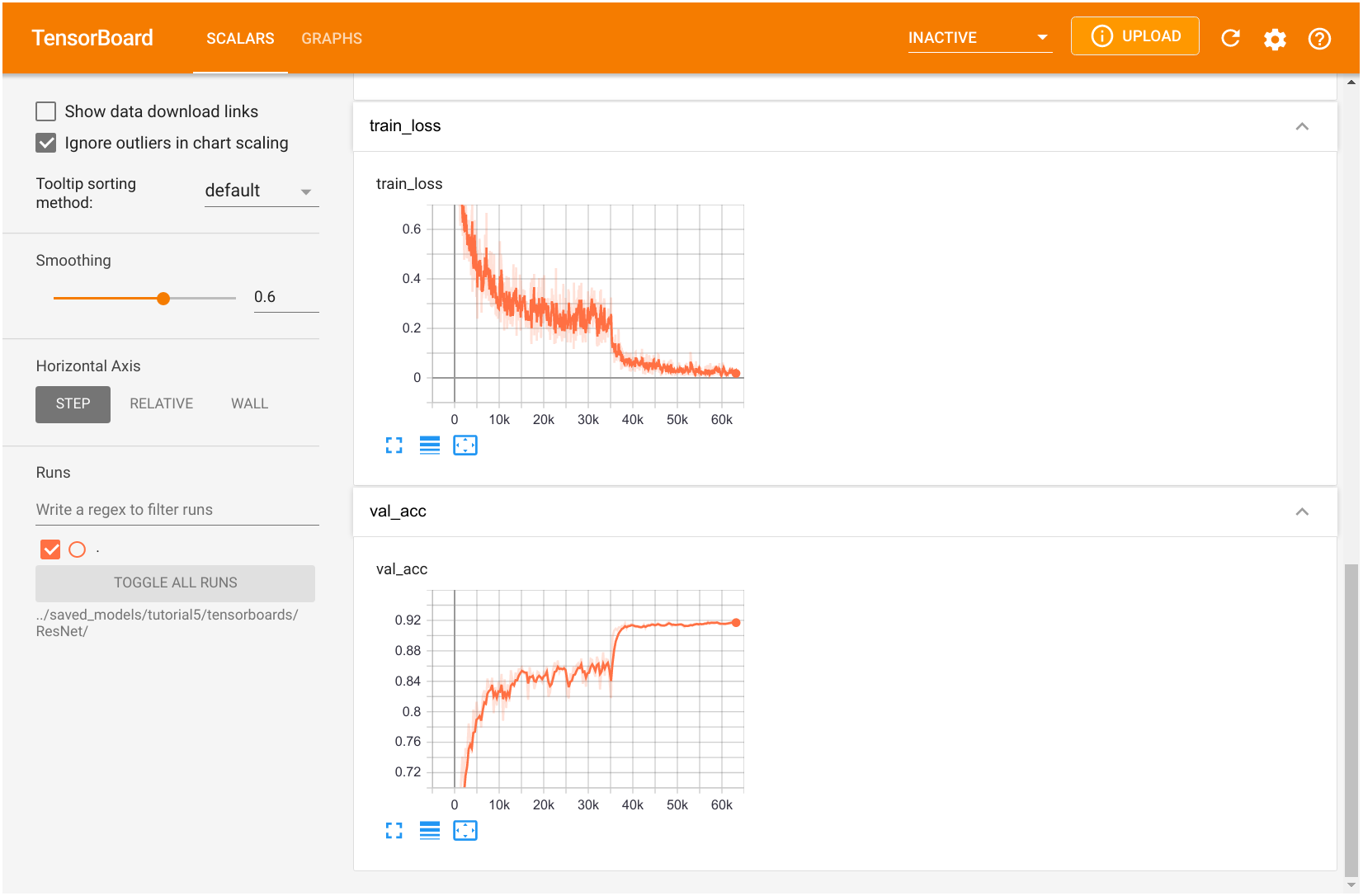
图6：ResNet模型训练的TensorBoard可视化展示

您可以自由探索 TensorBoard，包括计算图。一般来说，我们可以看到，在训练的第一阶段，使用 SGD 的 ResNet 的训练损失比 GoogleNet 高。然而，在降低学习率之后，模型的验证准确率更高。我们在笔记本的末尾比较了精确度得分。

2.3 DenseNet

2.3.1 DenseBlock

DenseNet是另一个用于支持非常深度神经网络的架构，它对残差连接采取了略有不同的视角。DenseNet不建模层之间的差异，而是将残差连接视为跨层重用特征的一种可能方式，从而消除了学习冗余特征图的任何必要性。如果我们深入网络，模型会学习抽象特征来识别模式。然而，一些复杂的图案由抽象特征（例如手、脸等）和低级特征（例如边缘、基本颜色等）的组合组成。为了在深层找到这些低级特征，标准的CNN必须学习复制这样的特征图，这浪费了大量的参数复杂度。DenseNet提供了一种高效的重用特征的方法，它让每个卷积依赖于之前的所有输入特征，但只向其添加少量的滤波器。请参见下图以获取说明：

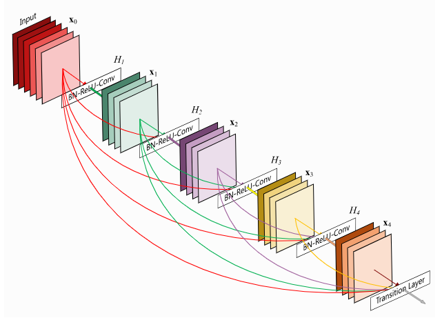
图7：DenseNet模型结构图

最后一层称为过渡层，负责在高度、宽度和通道大小上降低特征图的维数。虽然从技术上讲，它们打破了恒等式反向传播，但网络中只有几个，所以它不会对梯度流产生太大影响。

我们将DenseNet中层的实现拆分为三部分：一个DenseLayer，一个DenseBlock，一个TransitionLayer。模块DenseLayer在稠密块内实现单层。它应用1x1卷积与后续的3x3卷积进行降维。将输出通道串联到原始并返回。请注意，我们应用Batch Normalization作为每个块的第一层。这允许对不同层的相同特征进行略有不同的激活，具体取决于所需的内容。总体来说，我们可以这样实现：

class DenseLayer(nn.Module):
    
    def __init__(self, c_in, bn_size, growth_rate, act_fn):
        """
        Inputs:
            c_in - Number of input channels
            bn_size - Bottleneck size (factor of growth rate) for the output of the 1x1 convolution. Typically between 2 and 4.
            growth_rate - Number of output channels of the 3x3 convolution
            act_fn - Activation class constructor (e.g. nn.ReLU)
        """
        super().__init__()
        self.net = nn.Sequential(
            nn.BatchNorm2d(c_in),
            act_fn(),
            nn.Conv2d(c_in, bn_size * growth_rate, kernel_size=1, bias=False),
            nn.BatchNorm2d(bn_size * growth_rate),
            act_fn(),
            nn.Conv2d(bn_size * growth_rate, growth_rate, kernel_size=3, padding=1, bias=False)
        )
        
    def forward(self, x):
        out = self.net(x)
        out = torch.cat([out, x], dim=1)
        return out

模块DenseBlock总结了按顺序应用的多个密集层。每个密集层以原始输入和所有前一层的特征图作为输入：

class DenseBlock(nn.Module):
    
    def __init__(self, c_in, num_layers, bn_size, growth_rate, act_fn):
        """
        Inputs:
            c_in - Number of input channels
            num_layers - Number of dense layers to apply in the block
            bn_size - Bottleneck size to use in the dense layers
            growth_rate - Growth rate to use in the dense layers
            act_fn - Activation function to use in the dense layers
        """
        super().__init__()
        layers = []
        for layer_idx in range(num_layers):
            layers.append(
                DenseLayer(c_in=c_in + layer_idx * growth_rate, # Input channels are original plus the feature maps from previous layers
                           bn_size=bn_size,
                           growth_rate=growth_rate,
                           act_fn=act_fn)
            )
        self.block = nn.Sequential(*layers)
        
    def forward(self, x):
        out = self.block(x)
        return out

最后，TransitionLayer 将密集块的最终输出作为输入，并使用 1x1 卷积减少其通道维度。为了减少高度和宽度维度，我们采取了与 ResNet 不同的方法，应用了核大小为 2 和步幅为 2 的平均池化。这是因为我们在输出中没有额外的连接，而是考虑了完整的 2x2 补丁，而不是单个值。此外，与使用步幅为 2 的 3x3 卷积相比，这种方法更高效。因此，该层实现如下：

class TransitionLayer(nn.Module):
    
    def __init__(self, c_in, c_out, act_fn):
        super().__init__()
        self.transition = nn.Sequential(
            nn.BatchNorm2d(c_in),
            act_fn(),
            nn.Conv2d(c_in, c_out, kernel_size=1, bias=False),
            nn.AvgPool2d(kernel_size=2, stride=2) # Average the output for each 2x2 pixel group
        )
        
    def forward(self, x):
        return self.transition(x)

现在我们可以把所有东西放在一起，创建我们的 DenseNet。为了指定层数，我们使用与 ResNet 类似的符号，并传递一个整数列表，表示每个块的层数。在每个密集块之后，除了最后一个块之外，我们应用一个过渡层，将维度减少 2。

class DenseNet(nn.Module):
    
    def __init__(self, num_classes=10, num_layers=[6,6,6,6], bn_size=2, growth_rate=16, act_fn_name="relu", **kwargs):
        super().__init__()
        self.hparams = SimpleNamespace(num_classes=num_classes,
                                       num_layers=num_layers,
                                       bn_size=bn_size,
                                       growth_rate=growth_rate,
                                       act_fn_name=act_fn_name,
                                       act_fn=act_fn_by_name[act_fn_name])
        self._create_network()
        self._init_params()
        
    def _create_network(self):
        c_hidden = self.hparams.growth_rate * self.hparams.bn_size # The start number of hidden channels
        
        # A first convolution on the original image to scale up the channel size
        self.input_net = nn.Sequential(
            nn.Conv2d(3, c_hidden, kernel_size=3, padding=1) # No batch norm or activation function as done inside the Dense layers
        )
        
        # Creating the dense blocks, eventually including transition layers
        blocks = []
        for block_idx, num_layers in enumerate(self.hparams.num_layers):
            blocks.append( 
                DenseBlock(c_in=c_hidden, 
                           num_layers=num_layers, 
                           bn_size=self.hparams.bn_size,
                           growth_rate=self.hparams.growth_rate,
                           act_fn=self.hparams.act_fn)
            )
            c_hidden = c_hidden + num_layers * self.hparams.growth_rate # Overall output of the dense block
            if block_idx < len(self.hparams.num_layers)-1: # Don't apply transition layer on last block
                blocks.append(
                    TransitionLayer(c_in=c_hidden,
                                    c_out=c_hidden // 2,
                                    act_fn=self.hparams.act_fn))
                c_hidden = c_hidden // 2
                
        self.blocks = nn.Sequential(*blocks)
        
        # Mapping to classification output
        self.output_net = nn.Sequential(
            nn.BatchNorm2d(c_hidden), # The features have not passed a non-linearity until here.
            self.hparams.act_fn(),
            nn.AdaptiveAvgPool2d((1,1)),
            nn.Flatten(),
            nn.Linear(c_hidden, self.hparams.num_classes)
        )

    def _init_params(self):
        # Based on our discussion in Tutorial 4, we should initialize the convolutions according to the activation function
        for m in self.modules():
            if isinstance(m, nn.Conv2d):
                nn.init.kaiming_normal_(m.weight, nonlinearity=self.hparams.act_fn_name)
            elif isinstance(m, nn.BatchNorm2d):
                nn.init.constant_(m.weight, 1)
                nn.init.constant_(m.bias, 0)

    def forward(self, x):
        x = self.input_net(x)
        x = self.blocks(x)
        x = self.output_net(x)
        return x

我们还可以将DenseNet添加到我们的模型字典中：

model_dict["DenseNet"] = DenseNet

最后，我们训练我们的网络。与 ResNet 不同，DenseNet 在使用 Adam 优化器时没有出现任何问题，因此我们使用该优化器训练它。其他超参数的选择是为了使网络参数大小与 ResNet 和 GoogleNet 相似。通常，在设计非常深的网络时，DenseNet 比 ResNet 更高效，同时性能相似甚至更好。

densenet_model, densenet_results = train_model(model_name="DenseNet", 
                                               model_hparams={"num_classes": 10,
                                                              "num_layers": [6,6,6,6],
                                                              "bn_size": 2,
                                                              "growth_rate": 16,
                                                              "act_fn_name": "relu"}, 
                                               optimizer_name="Adam",
                                               optimizer_hparams={"lr": 1e-3,
                                                                  "weight_decay": 1e-4})

2.3.2 Tensorboard日志

最后，我们还有另一个用于DenseNet训练的TensorBoard。

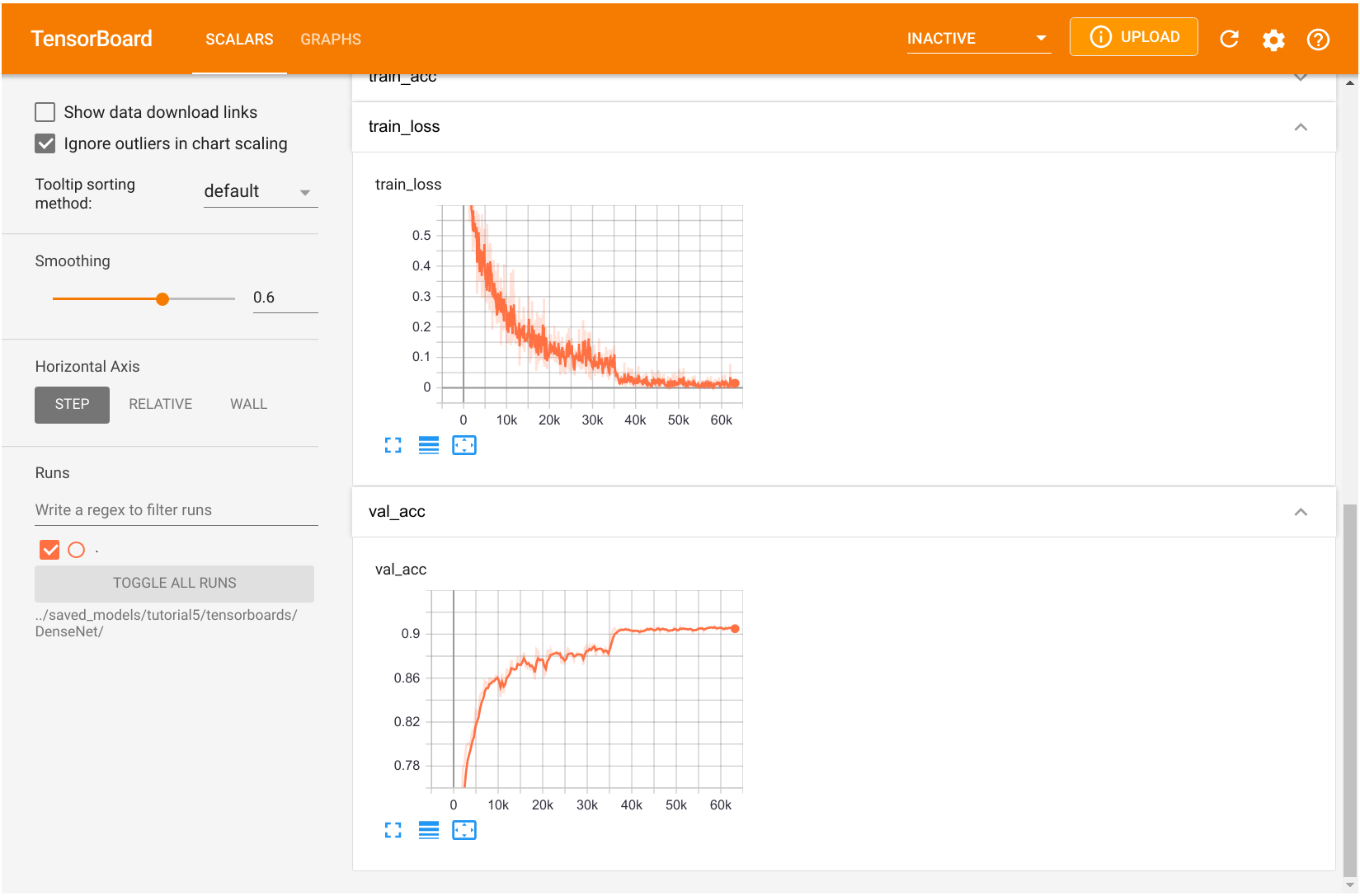
图8：DenseNet模型训练的TensorBoard可视化展示

验证准确率和训练损失的整体趋势与 GoogleNet 的训练相似，这也与使用 Adam 训练网络有关。您可以自由探索训练指标。

2.4 结论和比较

在分别讨论每个模型并训练所有模型之后，我们终于可以比较它们了。首先，让我们将所有模型的结果组织成一个表格：

%pip install tabulate

%%html
<!-- Some HTML code to increase font size in the following table -->
<style>
th {font-size: 120%;}
td {font-size: 120%;}
</style>

import tabulate
from IPython.display import display, HTML
all_models = [
    ("GoogleNet", googlenet_results, googlenet_model),
    ("ResNet", resnet_results, resnet_model),
    ("ResNetPreAct", resnetpreact_results, resnetpreact_model),
    ("DenseNet", densenet_results, densenet_model)
]
table = [[model_name,
          f"{100.0*model_results['val']:4.2f}%",
          f"{100.0*model_results['test']:4.2f}%",
          "{:,}".format(sum([np.prod(p.shape) for p in model.parameters()]))]
         for model_name, model_results, model in all_models]
display(HTML(tabulate.tabulate(table, tablefmt='html', headers=["Model", "Val Accuracy", "Test Accuracy", "Num Parameters"])))

Or 采用python 命令行方式输出：

import tabulate
import numpy as np  # 确保导入numpy（原代码中使用了np.prod）
# 假设all_models中的结果和模型已定义（需保留原有变量定义）
all_models = [
    ("GoogleNet", googlenet_results, googlenet_model),
    ("ResNet", resnet_results, resnet_model),
    ("ResNetPreAct", resnetpreact_results, resnetpreact_model),
    ("DenseNet", densenet_results, densenet_model)
]
# 构建表格数据（与原逻辑一致）
table = [
    [
        model_name,
        f"{100.0 * model_results['val']:4.2f}%",
        f"{100.0 * model_results['test']:4.2f}%",
        "{:,}".format(sum([np.prod(p.shape) for p in model.parameters()]))
    ]
    for model_name, model_results, model in all_models
]
# 命令行输出：使用适合终端的表格格式（如grid/fancy_grid）
print(tabulate.tabulate(
    table,
    headers=["Model", "Val Accuracy", "Test Accuracy", "Num Parameters"],
    tablefmt="fancy_grid"  # 终端友好的表格格式，可根据需要调整
))

在这里插入图片描述

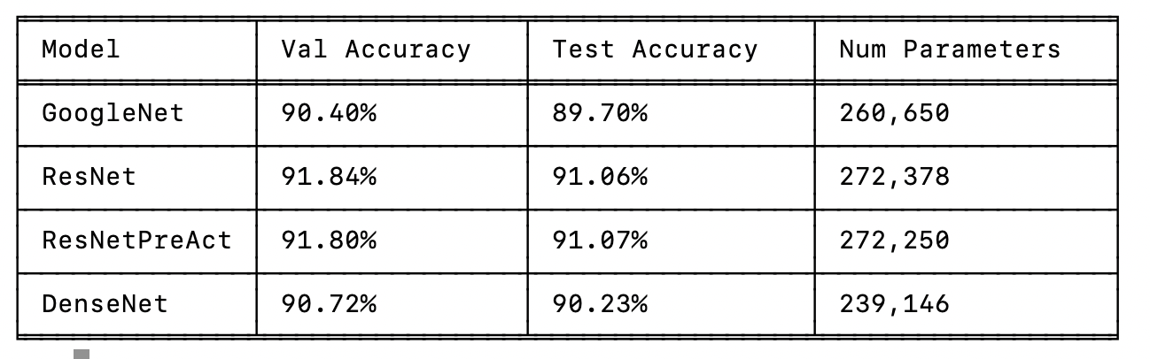
首先，我们看到所有模型的表现都相当不错。您在实践中实现的简单模型性能显著较低，这除了参数数量较少外，还归因于架构设计的选择。GoogleNet 是在验证集和测试集上表现最差的模型，尽管它与 DenseNet 的差距很小。对 GoogleNet 中的所有通道大小进行适当的超参数搜索可能会将模型的准确性提高到类似的水平，但由于超参数数量庞大，这也会很昂贵。ResNet 在验证集上的表现比 DenseNet 和 GoogleNet 高出 1% 以上，而原始版本和预激活版本之间的差异很小。我们可以得出结论，对于浅层网络，激活函数的位置似乎并不重要，尽管有论文报告了相反的情况。

总体而言，我们可以得出结论，ResNet 是一种简单但强大的架构。如果我们将这些模型应用于更复杂的任务，使用更大的图像和网络中的更多层，我们可能会看到 GoogleNet 和像 ResNet 和 DenseNet 这样的跳过连接架构之间的差距更大。有趣的是，DenseNet 在他们的设置中优于原始 ResNet，但与预激活 ResNet 非常接近。最佳模型，一种双路径网络，实际上是 ResNet 和 DenseNet 的结合，表明两者都提供了不同的优势。