tensorflow入门

最新推荐文章于 2024-02-01 15:12:40 发布

Waitfou

最新推荐文章于 2024-02-01 15:12:40 发布

阅读量4.1k

点赞数 2

分类专栏：深度学习

深度学习专栏收录该内容

6 篇文章 1 订阅

订阅专栏

本文转载自： tensorflow入门实战

TensorFlow计算模型-计算图

上一节我们讲到，TensorFlow中所有的计算都会被转换为计算图上的节点。如果说TensorFlow的Tensor是计算图的数据结构，那么Flow则体现了它的计算模型。我们这里详细了解一下计算图的使用.

计算图的简单示例

通过变量实现神经网络前向传播过程

#  coding:utf8

    import tensorflow as tf

    #声明w1,w2两个变量,这里还通过seed参数设定随机种子,保证每次运行结果一致
    w1 = tf.Variable(tf.random_normal([2, 3], stddev=1, seed=1))
    w2 = tf.Variable(tf.random_normal([3, 1], stddev=1, seed=1))

    #x设置为一个占位符
    x = tf.placeholder(tf.float32, shape=(None, 2), name='input')

    #矩阵乘法操作
    a = tf.matmul(x, w1)
    y = tf.matmul(a, w2)

    #创建一个会话
    sess = tf.Session()

    #初始化w1,w2
    sess.run(w1.initializer)
    sess.run(w2.initializer)

    #使用sess计算前向传播输出值
    print(sess.run(y, feed_dict={x: [[0.7, 0.9]]}))

    sess.close()
 
 1
2
3
4
5
6
7
8
9
10
11
12
13
14
15
16
17
18
19
20
21
22
23
24
25
26

从上述程序可以看出，使用一个图，简单的分为以下两步:

创建图结构(定义变量/计算节点)
创建会话，计算图

计算图的使用

TensorFlow程序一般分为两个阶段，第一阶段定义计算图中所有的计算。第二阶段为执行计算。

在编写程序过程中，TensorFlow会自动将定义的计算转化为计算图上的节点，在TensorFlow中，系统会自动维护一个默认的计算图，通过tf.get_default_graph函数可以获取当前默认的计算图。

    import tensorflow as tf
    a = tf.constant([1.0,2.0],name='a')
    b = tf.constant([2.0,3.0],name='b')
    result = a + b

    #通过a.graph可以查看张量所属的计算图，因为没有特意指定，所以这个计算图应该是默认的计算图
    print(a.graph is tf.get_default_graph())
    >>>True 
 
 1
2
3
4
5
6
7
8

创建新的计算图

除了使用默认的计算图，TensorFlow支持通过tf.Graph函数生成新的计算图。使用tf.Graph.as_default()方法将一个计算图设置为默认计算图，同时返回一个上下文管理器。这里可以配合with语句是保证操作的资源可以正确的打开和释放。不同的计算图上的张量和运算不会共享。。下面代码示意在不同计算图上定义和使用变量：

    # coding:utf8

    import tensorflow as tf

    g1 = tf.Graph()
    with g1.as_default():
        #在g1中定义v
        v = tf.get_variable("v",shape=[1],initializer=tf.zeros_initializer())


    g2 = tf.Graph()
    with g2.as_default():
        #在g2中定义v
        v = tf.get_variable("v",shape=[1],initializer=tf.ones_initializer())


    with tf.Session(graph=g1) as sess:
        tf.global_variables_initializer().run()
        with tf.variable_scope("",reuse=True):
            #在g1中,变量v取值应该为0,下面输出应该为[0.]
            print(sess.run(tf.get_variable('v')))


    with tf.Session(graph=g2) as sess:
        tf.global_variables_initializer().run()
        with tf.variable_scope("",reuse=True):
            #在g2中,变量v取值应该为1,下面输出应该为[1.]
            print(sess.run(tf.get_variable('v')))


    [ 0.]  #g1初始化为0
    [ 1.]  #g2初始化为1
 
 1
2
3
4
5
6
7
8
9
10
11
12
13
14
15
16
17
18
19
20
21
22
23
24
25
26
27
28
29
30
31
32

管理计算图等资源

TensorFlow还提供了管理Tensor和计算的机制，计算图可以通过tf.Graph.device函数来指定运行计算的设备。下面程序将加法计算放在GPU上执行。

g = tf.Graph()
    with g.device('/gpu:0'):
        result = a + b
 
 1
2
3

TensorFlow可以通过集合(collection)来管理不同类别的资源。例如使用tf.add_to_collection函数可以将资源加入一个或多个集合。使用tf.get_collection获取一个集合里面的所有资源。这些资源可以是张量/变量或者运行Tensorflow程序所需要的资源。（在神经网络的训练中会大量使用集合管理技术）

集合名称	集合内容	使用场景
tf.GraphKeys.GLOBAL_VARIABLES	所有变量	持久化Tensorflow模型
tf.GraphKeys.TRAINABLE_VARIABLES	可学习的变量(神经网络的参数)	模型训练/生成模型可视化内容
tf.GraphKeys.SUMMARIES	日志生成相关的张量	Tensorflow计算可视化
tf.GraphKeys.QUEUE_RUNNERS	处理输入的QueueRunner	输入处理
tf.GraphKeys.MOVING_AVERAGE_VARIABLES	所有计算了滑动平均值的变量	计算变量的滑动平均值

图相关的api函数

官方api地址点击这里
### Core graph data structures（class tf.Graph类的函数）

操作	description
tf.Graph.init()	创建一个空图
tf.Graph.as_default()	设置为默认图,返回一个上下文管理器(配合with关键字使用). 使用示例: g = tf.Graph() with g.as_default(): c = tf.constant(5.0)
tf.Graph.as_graph_def(from_version=None)	返回一个序列化的GraphDef对象序列化的GraphDef可以导入(使用import_graph_def())到其他Graph中或者被C++ Session API调用
tf.Graph.finalize()	完成图的构建，将图设置为只读(调用后任何ops都加入不到graph里)
tf.Graph.finalized	True if this graph has been finalized.
tf.Graph.control_dependencies(control_inputs)	指定一个带有control_dependencies的上下文管理器(配合with指定ops对control_inputs的依赖) `with g.control_dependencies([a, b, c]): # dandewill only run after a, b, and chave executed. d = … e = …`
tf.Graph.device(device_name_or_fuc)	返回一个指定使用device的上下文管理器. 参数 device_name_or_fuc可为:device name string/a device function/None with g.device(‘/gpu:0’):.. #设置程序运行在gpu上
tf.Graph.name_scope(name)	返回为ops创建层次名称(hierarchical names)的上下文管理器 (常用用来控制管理神经网络的权重变量,便于迭代更新计算等操作)
tf.Graph.add_to_collection(name, value)	将value以name放置到collection中(利用collection机制管理变量等)
tf.Graph.get_collection(name, scope=None)	从collection返回name的元素列表
tf.Graph.as_graph_element(obj, allow_tensor=True, allow_operation=True)	Returns the object referred to by obj, as an Operation or Tensor.
tf.Graph.get_operation_by_name(name)	Returns the Operation with the given name
tf.Graph.get_tensor_by_name(name)	Returns the Tensor with the given name.
tf.Graph.get_operations()	返回图中ops列表
tf.Graph.get_default_device()	Returns the default device.
tf.Graph.seed
tf.Graph.unique_name(name)	Return a unique Operation name for “name”.
tf.Graph.version	Returns a version number that increases as ops are added to the graph.
tf.Graph.create_op(op_type, inputs, dtypes, input_types=None, name=None, attrs=None, op_def=None, compute_shapes=True)	Creates an Operation in this graph. 这是一个low-level的创建ops的接口,大部分程序使用Python op constructors代替此函数 such as tf.constant(), 在默认图上添加一个ops.
tf.Graph.gradient_override_map(op_type_map)	测试中:返回一个带图梯度下降函数的上下文管理器

Tensorflow数据模型-张量

Tensor是TensorFlow管理数据的形式，从功能的角度上来看，Tensor可以简单的理解为多维数数组，其中零阶Tensor表示为标量(Scalar)，即一个数。但Tensor在TensorFlow中实现并不是直接采用数组的形式，而是对TensorFlow中运算结果的引用。Tensor保存是对如何得到数字的计算过程.
Tensor的用途分为两类：一是对中间计算结果的引用，这样方便获取中间计算结果同时提高了代码的阅读性。二是可以用来获得计算结果，这需要配合session.
以下示例程序:

    # coding:utf8

    import tensorflow as tf

    a = tf.constant([1.0,2.0],name='a')
    b = tf.constant([2.0,3.0],name='b')

    result = tf.add(a,b,name='add')

    print(result)

    #输出
    Tensor("add:0", shape=(2,), dtype=float32)
    #这是一个张量结构,需要配合session使用才能计算出结果
 
 1
2
3
4
5
6
7
8
9
10
11
12
13
14

张量结构

以上述程序为例，一个Tensor的结构为

Tensor("add:0", shape=(2,), dtype=float32)
 
 1

这其中主要包含了三个属性:name/shape/type(标识/维度/类型).

name属性

name是一个Tensor的唯一标识符，同时name也给出了该Tensor是如何计算出来的。计算图上的node和计算是相对应的。
计算的结果保存在Tensor中，Tensor的name属性可以通过”node:src_output”形式给出。

node为节点的名称-
src_output表示Tensor来自当前节点的第几个输出。

例如上述程序的

Tensor("add:0", shape=(2,), dtype=float32)
#name为"add:0"即 表示node的ops为add 且是第0个输出.
 
 1
2

shape属性

shape属性描述了一个Tensor的维度信息，维度是Tensor一个极其重要的属性，后面学习过程会有大量操作维度的计算。
在程序中:

Tensor("add:0", shape=(2,), dtype=float32)
#"shape=(2,)"说明result是一个一维向量，向量的长度为2.
 
 1
2

type属性

每一个Tensor都有一个唯一的类型，TensorFlow会对所有参与计算的Tensor进行类型检查，当发现类型不匹配时会报错。
例如：

import tensorflow as tf

    a = tf.constant([1,2],name='a')   #检测为int32
    b = tf.constant([2.0,3.0],name='b') #检测为float32
    result = a + b

    # result = a + b
    # ValueError: Tensor conversion requested dtype int32 for Tensor with dtype float32: 'Tensor("b:0", shape=(2,), dtype=float32)'
 
 1
2
3
4
5
6
7
8

这里对常量a默认为int32类型，在与float32类型的b相加会出现类型不匹配，故报错.

我们可以指定constant的类型，例如将a改为float32类型，例如下面程序就不会报错了

import tensorflow as tf

    a = tf.constant([1,2],name='a',dtype=tf.float32) #dtype='float32'也可以，为了兼容性，最好还是tf.float32
    b = tf.constant([2.0,3.0],name='b')

    result = a + b
 
 1
2
3
4
5
6

TensorFlow中types相关属性

在TensorFlow中有14种不同的类型,见下表

类型	描述符
实数	tf.float32 : 32-bit single-precision floating-point. tf.float64: 64-bit double-precision floating-point. tf.bfloat16: 16-bit truncated floating-point.
整数	tf.int8: 8-bit signed integer. tf.uint8: 8-bit unsigned integer tf.int32: 32-bit signed integer tf.int64: 64-bit signed integer. tf.qint8: Quantized 8-bit signed integer. tf.quint8: Quantized 8-bit unsigned integer tf.qint32: Quantized 32-bit signed integer
布尔	tf.bool: Boolean.
复数	tf.complex64: 64-bit single-precision complex.

type的api（class tf.DType）

操作	description
tf.DType.is_compatible_with(other)	如果other类型可以转为为此类型，返回True
tf.DType.name	Returns the string name for this DType.
tf.DType.base_dtype	Returns a non-reference DType based on this DType.
tf.DType.is_ref_dtype	Returns True if this DType represents a reference type.
tf.DType.as_ref	Returns a reference DType based on this DType.
tf.DType.is_integer	Returns whether this is a (non-quantized) integer type.
tf.DType.is_quantized	Returns whether this is a quantized data type.
tf.DType.as_numpy_dtype	Returns a numpy.dtype based on this DType
tf.DType.as_datatype_enum	Returns a types_pb2.DataType enum value based on this DType.
tf.DType.init(type_enum)	Creates a new DataType.
tf.DType.max	Returns the maximum representable value in this data type.
tf.DType.min	Returns the minimum representable value in this data type.
tf.as_dtype(type_value)	Converts the given type_value to a DType.

张量相关api

class tf.Tensor
Represents a value produced by an Operation.

A Tensor is a symbolic handle to one of the outputs of an Operation. It does not hold the values of that operation’s output, but instead provides a means of computing those values in a TensorFlow Session.

This class has two primary purposes:

A Tensor can be passed as an input to another Operation. This builds a dataflow connection between operations, which enables TensorFlow to execute an entire Graph that represents a large, multi-step computation.
After the graph has been launched in a session, the value of the Tensor can be computed by passing it to Session.run(). t.eval() is a shortcut for calling tf.get_default_session().run(t).

操作	description
tf.Tensor.dtype	Tensor的DType属性
tf.Tensor.name	Tensor的Name属性
tf.Tensor.value_index	Tensor在对应的ops(即创建tensor的ops)输出序号
tf.Tensor.graph	包含该tensor的计算图
tf.Tensor.op	创建该Tensor的ops
tf.Tensor.consumers()	返回使用该Tensor的ops列表
tf.Tensor.eval(feed_dict=None, session=None)	在session中计算Tensor值该函数要再session中使用,即with sess.as_default() 或者eval(session=sess)指定sess对象
tf.Tensor.get_shape()	返回类型为TensorShape的Tensor的shape
tf.Tensor.set_shape(shape)	更新Tensor的Shape
tf.Tensor.init(op, value_index, dtype)	Creates a new Tensor
tf.Tensor.device	设置计算该Tensor的设备

会话(Session)

会话(Session)拥有并管理TensorFlow运行时的所有资源，同时每个会话有自己的资源，例如 tf.Variable, tf.QueueBase, and tf.ReaderBase.当这些资源使用完毕后，及时的释放这些资源是很重要的,此时可以使用Session.close释放会话资源.，当所有计算完成后需要关闭会话来帮助系统回收资源，避免资源泄漏等问题。

会话模式

TensorFlow使用会话模式一般分为两种，明确调用会话生成函数和通过上下文管理器管理会话.

1.会话模式–明确调用会话生成函数和关闭会话函数

使用这种模式，当所有计算完成后，需要使用session.close函数关闭会话释放资源，当程序出现异常，会话得不到正常关闭。使用示例如下：

    #创建一个会话
    sess = tf.Session()

    #使用这个会话可以得到张量的结果,例如sess.run(result)
    sess.run(...)

    #关闭会话
    sess.close()
 
 1
2
3
4
5
6
7
8

2.会话模式–通过Python上下文管理器

在Python中，我们常使用上下文管理器来操作文件，例如

    with open('...') as fp: 
 
 1

这样做的好处，是利用上下文管理器来帮助我们简化操作，保证资源的有效利用和释放.同样的我们也可以使用with来操作Session.

    #创建一个会话,通过上下文管理器管理会话
    with tf.Session() as sess:
        #do what you want
        sess.run(...)

    #用完了就不用管了
 
 1
2
3
4
5
6

默认会话

TensorFlow在管理计算图时会自动生成一个默认的计算图，会话也有类似的机制，但需要手动指定。当默认的会话被指定之后可以通过tf.Tensor.eval函数来计算一个张量的取值.例如

sess = tf.Session()
    with sess.as_default():
        print(result.eval()) #计算张量的结果
 
 1
2
3

或者代码这样写

    sess = tf.Session()

    #下面两个功能一样
    print(sess.run(result))
    print(result.eval(session=sess))
 
 1
2
3
4
5

在交互式环境中，通过设置默认会话的方式获取张量的结果更加容易.TensorFlow提供了一种在交互式环境下直接构造默认会话的函数，即tf.InteractiveSession,用法如下

    sess = tf.InteractiveSession()
    print(result.eval())  #通过tf.InteractiveSession可以省去注册默认会话的操作
    sess.close()
 
 1
2
3

tf.InteractiveSession相关api（class tf.InteractiveSession）

A TensorFlow Session for use in interactive contexts, such as a shell.
The only difference with a regular Session is that an InteractiveSession installs itself as the default session on construction. The methods tf.Tensor.eval and tf.Operation.run will use that session to run ops.

操作	description
graph	The graph that was launched in this session.
graph_def	A serializable version of the underlying TensorFlow graph
init(target=”,graph=None,config=None)	Creates a new interactive TensorFlow session
as_default()	设置为默认Session,并返回这个上下文管理器.
close()	Closes an InteractiveSession.
make_callable(fetches,feed_list=None)	Returns a Python callable that runs a particular step.
partial_run(handle,fetches, feed_dict=None)	Continues the execution with more feeds and fetches.
partial_run_setup(fetches,feeds=None)	Sets up a graph with feeds and fetches for partial run.
run(fetches,feed_dict=None,options=None,run_metadata=None)	执行一个ops并获取一个Tensor的值

配置会话属性

无论是用哪种方法产生的会话，都可以通过ConfigProto Protocol Buffer来配置需要生成的会话.方法如下:

   config = tf.ConfigProto(allow_soft_placement=True,log_device_placement=True)
   sess1 = tf.InteractiveSession(config=config)
   sess2 = tf.Session(config=config)
 
 1
2
3

通过ConfigProto可以配置类似并行线程数/GPU分配策略/运行超算时间等参数.
常用的两个参数:

第一个参数:allow_soft_placement

这是一个布尔型参数,当这个值为True，以下任意一个条件成立，GPU上的运算可以放到CPU上:
- 1.运行无法在GPU上执行
- 2.没有GPU资源(例如指定在第三GPU上运行，但是只有一个GPU)
- 3.运行输入包含对CPU结果的引用
这个参数默认为False，为了提供代码的可移植性，设置参数为True，可以将在GPU上不支持的运算调整到CPU上，而不是报错。

第二个参数:log_device_placement

这是一个布尔型参数，当设置为True时日志中将会记录每个节点被安排在哪个设备上以方便调试.

会话相关api（tf.Session）

A Session object encapsulates the environment in which Operation objects are executed, and Tensor objects are evaluated.

操作	description
graph	The graph that was launched in this session.
graph_def	A serializable version of the underlying TensorFlow graph.
sess_str
init(target=”,graph=None, config=None)	Creates a new TensorFlow session.
as_default()	Returns a context manager that makes this object the default session.
close()	Closes this session.
make_callable( fetches, feed_list=None)	Returns a Python callable that runs a particular step.
partial_run(handle,fetches,feed_dict=None)	Continues the execution with more feeds and fetches.
partial_run_setup( fetches,feeds=None)	Sets up a graph with feeds and fetches for partial run.
reset(target, containers=None,config=None)	Resets resource containers on target, and close all connected sessions.
run(fetches, feed_dict=None,options=None,run_metadata=None)	Runs operations and evaluates tensors in fetches.

TensorFlow变量

在TensorFlow中变量(tf.Variable)的作用可用保存和模型中参数,创建Variable需要传入一个初始化值，TensorFlow中变量初始值可以设置为随机数、常数或者是通过其他变量初始值计算得到。初始化时这需要指定Variable的type和shape(初始化过后Tensor的type和shape不可变，Value可以通过assign函数改变).如果需要动态的改变Variable的shape，在声明时指定validate_shape=False.）

下面代码给出了一种TensorFlow变量初始化.

import tensorflow as tf

# Create a variable.
w = tf.Variable(<initial-value>, name=<optional-name>)

#for example
weights = tf.Variable(tf.random_normal([2,3],stddev=2))
#使用tf.random_normal([2,3],stddev=2)产生一个2x3矩阵，矩阵中元素均为0，标准差为2的随机数。tf.random_normal函数可以通过参数mean来指定平均值，在没指定时默认为0.

# Use the variable in the graph like any Tensor.
y = tf.matmul(w, ...another variable or tensor...)

# The overloaded operators are available too.
z = tf.sigmoid(w + y)

# Assign a new value to the variable with `assign()` or a related method.
w.assign(w + 1.0)
w.assign_add(1.0)

 
 1
2
3
4
5
6
7
8
9
10
11
12
13
14
15
16
17
18
19

在操作图时，应明确的初始化所有变量.可以通过初始化ops完成变量的初始化.示意如下:

# Launch the graph in a session.
with tf.Session() as sess:
    # Run the variable initializer.
    sess.run(w.initializer)
    # ...you now can run ops that use the value of 'w'...



    #通过其他变量来初始化
    w2 = tf.Variable(weights.initialized_value())
    w3 = tf.Variable(weights.initialized_value()*2.0)
    #w2初始值设置为和weights变量相同,w3是weights的两倍
 
 1
2
3
4
5
6
7
8
9
10
11
12

通常大大多数初始化操作是使用global_variables_initializer()函数添加一个初始化ops，我们先运行初始化ops后再执行其他计算,global_variables_initializer()用法如下：

# Add an Op to initialize global variables.
init_op = tf.global_variables_initializer()

# Launch the graph in a session.
with tf.Session() as sess:
    # Run the Op that initializes global variables.
    sess.run(init_op)
    # ...you can now run any Op that uses variable values...
 
 1
2
3
4
5
6
7
8

所有的变量在创建时会自动收集到Collections，通常会被收集到GraphKeys.GLOBAL_VARIABLES中。使用global_variables()可以返回这个Collections的上下文。

在构建机器学习模型时，我们可以很方便的区别在训练模型不变Variable和其他Variable.例如用于记录训练次数的全局变量。为了简化操作，变量初始化时可以设置 trainable= parameter属性，如果设置为True，新的变量会添加到GraphKeys.TRAINABLE_VARIABLES,我们也可以使用trainable_variables()函数获取此Collections.The various Optimizer classes可以利用此Collections优化参数.

TensorFlow随机数生成函数

TensorFlow的Variable可以通过随机函数初始化，下面是TensorFlow中常用的随机函数:

函数名称	随机数分布	主要参数
tf.random_normal	正态分布	平均值/标准差/取值类型
tf.truncated_normal	正态分布，但如果随机出来的值偏离平均值超过2个标准差，这个数会被重新随机	平均值/标准差/取值类型
tf.random_uniform	平均分布	最小/最大取值/取值类型
tf.random_gamma	Gamma分布	形状参数alpha/尺度参数beta/取值类型

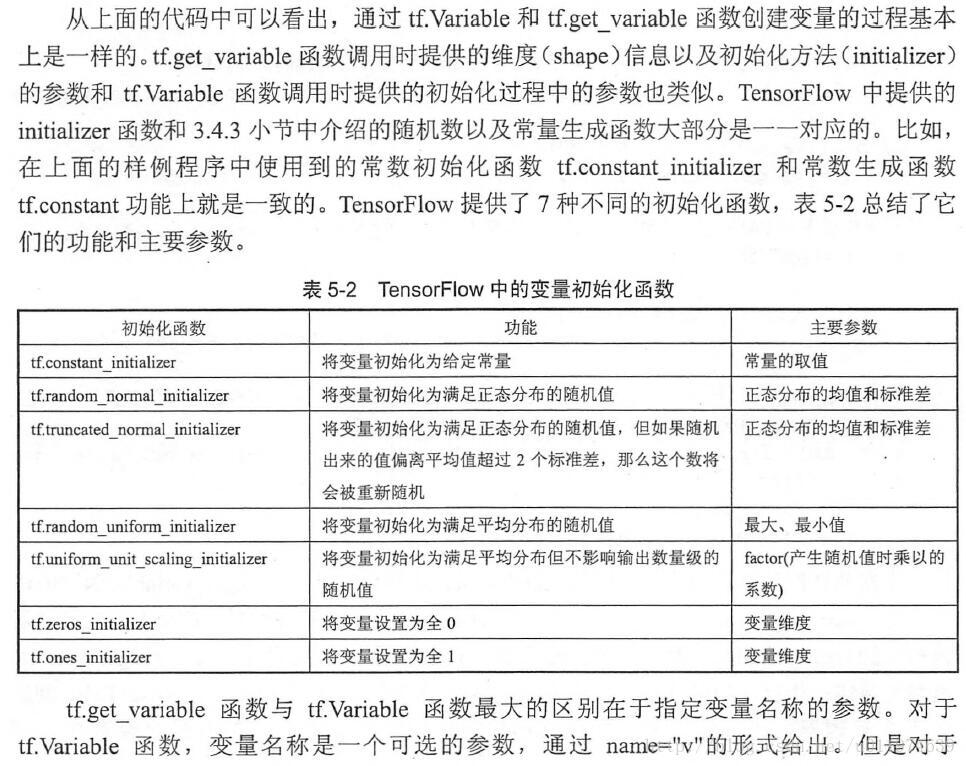
TensorFlow也支持通过常数来初始化一个变量。下表是TensorFlow中常用的常量声明方法.

函数名称	功能	样例
tf.zeros	全0数组	tf.zeros([2,3],int32)->[[0,0,0],[0,0,0]]
tf.ones	全1数组	tf.zeros([2,3],int32)->[[1,1,1],[1,1,1]]
tf.fill	产生一个全部为给定数字的数组	tf.zeros([2,3],9)->[[9,9,9],[9,9,9]]
tf.constant	产生一个给定值常量	tf.constant([1,2,3])->[1,2,3]

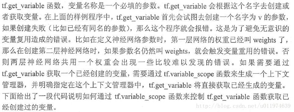
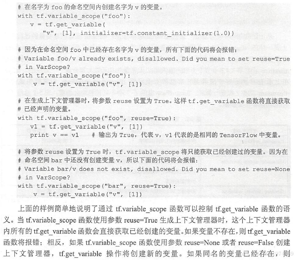
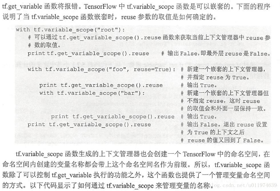
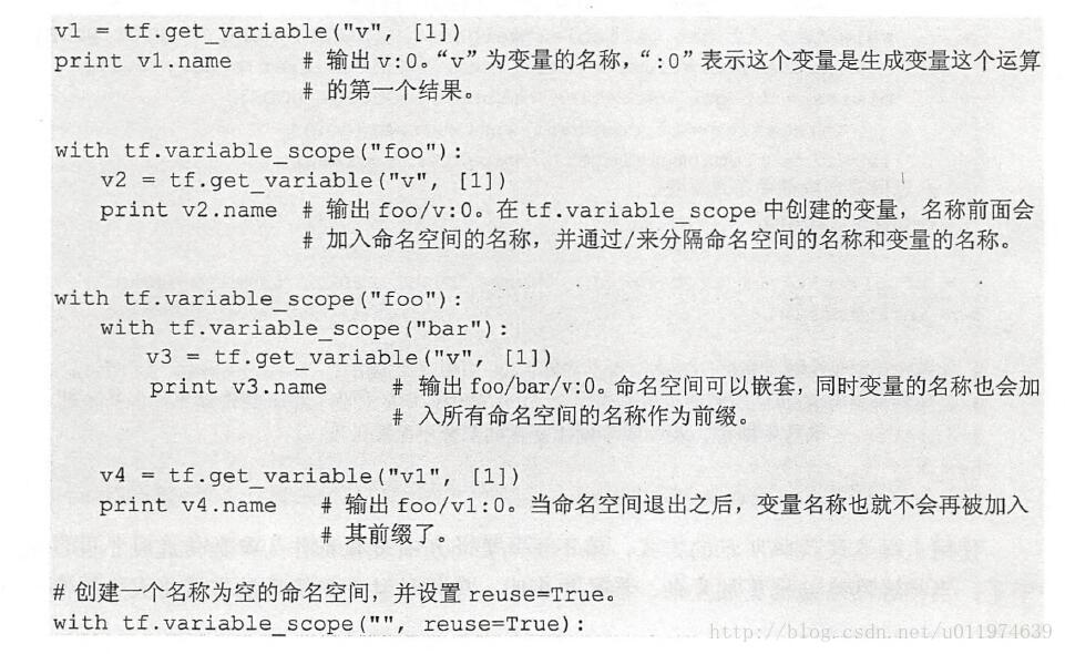
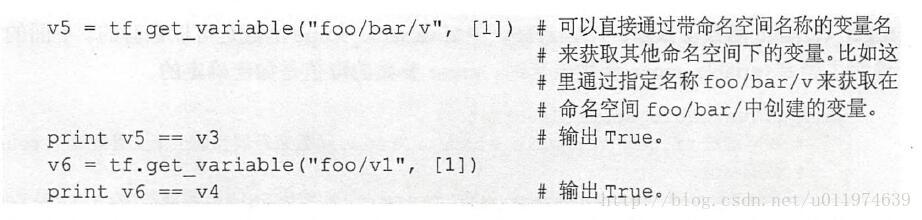
变量管理

TensorFlow提供了通过变量名称来创建或者获取一个变量的机制，通过这个机制，在不同的函数中可以直接通过变量的名字来使用变量，而不需要将变量通过参数的形式传递。
TensorFlow通过变量名称获取变量的机制主要通过tf.get_variable和tf.variable_scope函数实现.

创建Variable可通过Variable()也可以使用get_variable()。
以下代码是通过两个函数创建同一个变量的实例:

v =tf.get_variable("v",shape=[1],initializer=tf.constant_initializer(1.0))
v = tf.Variable(tf.constant(1.0,shape=[1],name='v')
 
 1
2

这里写图片描述

Variable的api(tf.Variable)

操作	description
device	The device of this variable.
dtype	The DType of this variable.
graph	he Graph of this variable.
initial_value	Returns the Tensor used as the initial value for the variable.
initializer	The initializer operation for this variable.
name	The name of this variable.
op	The Operation of this variable.
shape	The TensorShape of this variable.
init( initial_value=None, trainable=True, collections=None, validate_shape=True, caching_device=None, name=None, variable_def=None, dtype=None, expected_shape=None, import_scope=None )	使用initial_value创建一个新的Variable 如果trainable为True,则Variable会自动添加到GraphKeys.TRAINABLE_VARIABLES(可训练)*的Collecion collections:新变量会添加到该collections,默认会添加到GraphKeys.TRAINABLE_VARIABLES validate_shape:如果为False,允许变量以None指定shape caching_device:the Variable should be cached for reading. Defaults to the Variable’s device. name:Defaults to ‘Variable’ and gets uniquified automatically variable_def:VariableDef protocol buffer. dtype:If set, initial_value will be converted to the given type expected_shape:A TensorShape. If set, initial_value is expected to have this shape. import_scope:Name scope to add to the Variable. Only used when initializing from protocol buffer.
abs(a,*args)	绝对值
add_(a,*args)	x+y加(每个元素相加)
and(a,*args)	返回and操作结果(每个元素)
div(a,*args)	除
floordiv(a,*args)	Divides x / y elementwise
ge(a,*args)	返回x>=y的bool型矩阵
getitem(var,slice_spec)	Creates a slice helper object given a variable.
gt(a,*args)	返回x>y的bool型矩阵
invert(a,*args)	返回Not操作的bool矩阵
le(a,*args)	返回x<=y的bool型矩阵
lt(a,*args)	返回x
matmul(a,*args)	x与y的矩阵乘法
mod(a,*args)	取模
mul(a,*args)	Dispatches cwise mul for “DenseDense” and “DenseSparse”.
neg(a,*args)	去相反值
pow(a,*args)	computes xy
sub(a,*args)	x-y(每个元素)
xor(a,*args)	x ^ y = (x
assign(value,use_locking=False)	为Variable分配一个新值
assign_add(value,use_locking=False)	Adds a value to this variable.
assign_sub(value,use_locking=False)	Subtracts a value from this variable.
count_up_to(limit)	increments this variable until it reaches limit.
eval(session=None)	在session中计算Variable的Value
from_proto(variable_def, import_scope=None)	Returns a Variable object created from variable_def.
get_shape()	Alias of Variable.shape.
initialized_value()	初始化Variable
load(value, session=None)	Load new value into this variable Writes new value to variable’s memory. Doesn’t add ops to the graph
read_value()	返回Variable的Value
scatter_sub(sparse_delta,use_locking=False)	Subtracts IndexedSlices from this variable.
set_shape(shape)	Overrides the shape for this variable.
to_proto(export_scope=None)	Converts a Variable to a VariableDef protocol buffer.
value()	Returns the last snapshot of this variable

深度神经网络

TensorFlow神经网络介绍

在这里，我们结合神经网络的功能进一步的介绍如何通过TensorFlow来实现神经网络。首先我们使用TensorFlow游乐场(TensorFlow工具)简单了解实现神经网络的功能和计算流程。再使用TensorFlow实现神经网络的FP(前向传播)和BP(反向传播)算法.

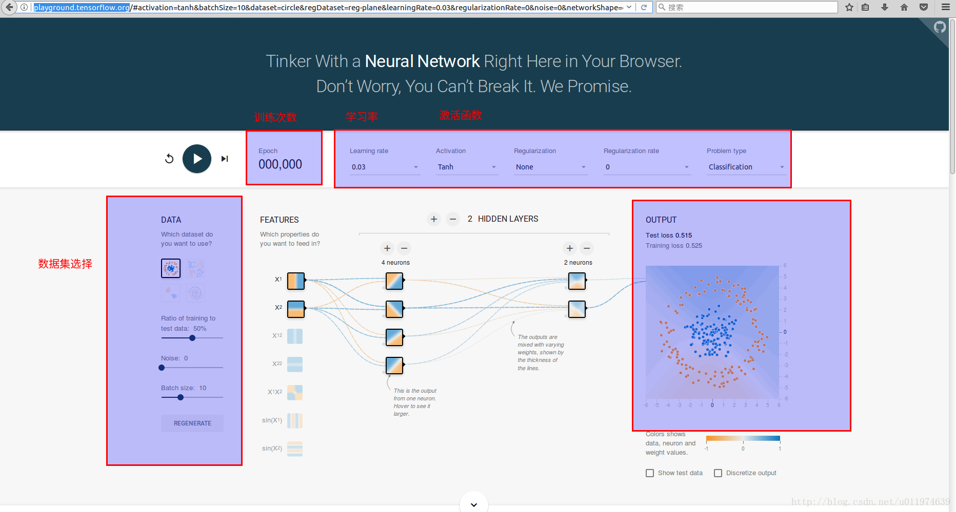
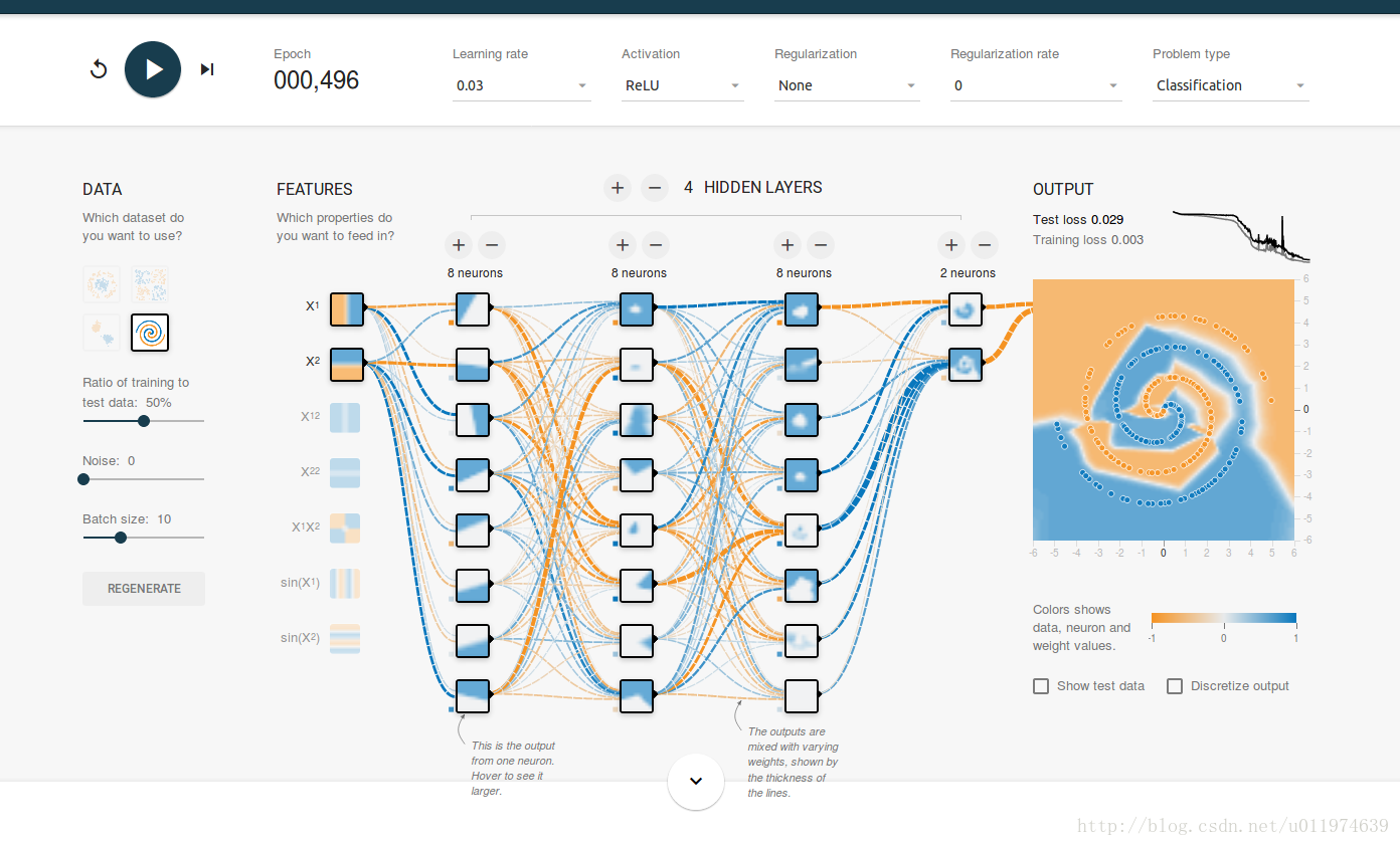
TensorFlow游乐场

TensorFlow游乐场(http://playground.tensorflow.org)是一个Web应用，可以训练简单的神经网络并实现可视化训练过程的工具.
这里写图片描述

使用神经网络解决分类问题主要分为一下4个步骤:

1.提取问题中实体的特征向量作为数据网络的输入
2.定义神经网络的结构，并定义如何从神经网络的输入得到输出
3.通过训练数据调整神经网络的参数取值
4.使用训练好的模型来预测未知的数据

这里写图片描述

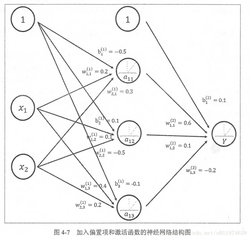
前向传播算法介绍

不同的神经网络结构前向传播的方式也不一样，这里介绍最简单的全连接网络结构的前向传播算法，之所以称为全连接神经网络是因为相邻两层之间任意两个节点都有链接.

这里写图片描述

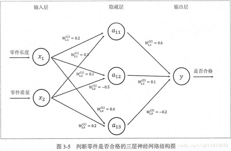
其中第一部分是神经网络的输入:从实体中提取的特征向量。图示为x1和x2
第二部分是神经网络的连接结构:节点a11/a12/a13和连接权值W矩阵，其中w的上标表明了神经网络的层数，下标表明了连接节点编号，比如w11即表示连接x1到a11的权值.(连接元素的具体位置取决与上标)

整个神经网络前向传播的过程
这里写图片描述

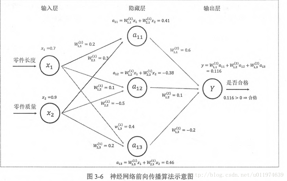
前向传播算法可以表示为矩阵乘法，将输入x1，x2，组织成一个1x2的矩阵X=[x1,x2]，而W组织成一个2x3的矩阵(矩阵行数为输入个数，矩阵列数为当前层节点个数):

这里写图片描述

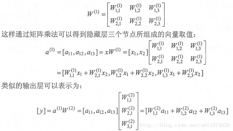
这样前向算法用矩阵方式表达出来了，在TensorFlow中矩阵乘法是很容易实现的。

     a = tf.matmul(x,w1)
     y = tf.matmul(a,w2)  #matmul实现矩阵乘法
 
 1
2

通过变量实现神经网络前向传播过程

代码如下


    #  coding:utf8

    import tensorflow as tf

    #声明w1,w2两个变量,这里还通过seed参数设定随机种子,保证每次运行结果一致
    w1 = tf.Variable(tf.random_normal([2, 3], stddev=1, seed=1))
    w2 = tf.Variable(tf.random_normal([3, 1], stddev=1, seed=1))

    #暂时将输入特征向量设置为一个变量
    x = tf.constant([[0.7, 0.9]])  #注意这里声明的是一个1x2的矩阵

    a = tf.matmul(x, w1)
    y = tf.matmul(a, w2)

    sess = tf.Session()

    sess.run(w1.initializer)
    sess.run(w2.initializer)

    #使用tf.initialize_all_variables()可以初始化多个变量
    #sess.run(tf.initialize_all_variables())

    print(sess.run(y))

    sess.close()
 
 1
2
3
4
5
6
7
8
9
10
11
12
13
14
15
16
17
18
19
20
21
22
23
24
25
26

输出为

[[ 3.95757794]]
 
 1

需要注意的地方有:

在声明好变量时，需要使用session初始化变量(run(w.initializer)或者使用run(tf.initialize_all_variables())初始化所有变量)
注意在声明输入x的时候,要初始化一个矩阵常量的方法
所有变量都会被自动的加入Grpah.VARIABLES集合。通过tf.variables函数可以得到当前计算图所有的变量

通过TensorFlow训练神经网络模型

在神经网络中，常用的方法是BP算法，下图是BP算法执行的流程图
这里写图片描述

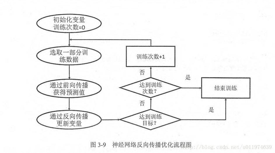
BP算法是一个迭代的过程，再每次迭代过程开始，取一小部分训练数据叫做一个batch.依据前向传播的输出值与标签值的差值做BP优化。
这里需要注意，上一节代码我们声明输入用的是x=tf.constant([[0.7,0.9]])，一般神经网络训练过程会需要多次迭代，每次迭代中选取的数据不能靠变量来表示，这里TensorFlow提供了placeholder机制用于输入数据，placeholder相当于定义一个位置，这个位置中的数据在程序运行时再指定。placeholder定义时，这个位置的数据类型需要指定而且不能改变。

使用placeholder

    #  coding:utf8

    import tensorflow as tf

    #声明w1,w2两个变量,这里还通过seed参数设定随机种子,保证每次运行结果一致
    w1 = tf.Variable(tf.random_normal([2, 3], stddev=1, seed=1))
    w2 = tf.Variable(tf.random_normal([3, 1], stddev=1, seed=1))

    #暂时将输入特征向量设置为一个变量
    x = tf.placeholder(tf.float32, shape=(1, 2), name='input')

    a = tf.matmul(x, w1)
    y = tf.matmul(a, w2)

    sess = tf.Session()

    sess.run(tf.initialize_all_variables())
    print(sess.run(y, feed_dict={x: [[0.7, 0.9]]}))
    sess.close()
 
 1
2
3
4
5
6
7
8
9
10
11
12
13
14
15
16
17
18
19

输出

[[ 3.95757794]]
 
 1

可以改变输入矩阵，得到n个样例的前向传播结果.例如:将输入改为3组数据

    #  coding:utf8

    import tensorflow as tf

    #声明w1,w2两个变量,这里还通过seed参数设定随机种子,保证每次运行结果一致
    w1 = tf.Variable(tf.random_normal([2, 3], stddev=1, seed=1))
    w2 = tf.Variable(tf.random_normal([3, 1], stddev=1, seed=1))

    #暂时将输入特征向量设置为一个变量
    x = tf.placeholder(tf.float32, shape=(3, 2), name='input')


    a = tf.matmul(x, w1)
    y = tf.matmul(a, w2)

    sess = tf.Session()

    sess.run(tf.initialize_all_variables())

    print(sess.run(y, feed_dict={x: [[0.7, 0.9], [0.1, 0.4], [0.5, 0.8]]}))

    sess.close()
 
 1
2
3
4
5
6
7
8
9
10
11
12
13
14
15
16
17
18
19
20
21
22

输出

    [[ 3.95757794]
     [ 1.15376532]
     [ 3.16749239]]
 
 1
2
3

再得到batch的前向传播结果后，需要定义损失函数刻画输出与标签值的差距，再通过BP调整网络参数。

    #定义损失函数
    cross_entropy = -tf.reduce_mean(y_*tf.log(tf.clip_by_value(y,1e-10,1.0)))

    #定义学习率
    learning_rate = 0.001

    #定义BP算法优化神经网络参数
    train_step = tf.train.AdamOptimizer(learning_rate).minimize(cross_entropy)
 
 1
2
3
4
5
6
7
8

cross_entropy定义了输出值和标签值的交叉熵，这是分类问题的一个常用的损失函数.
train_step定义了BP算法的优化方法，目前TensorFlow支持7种不同的优化器，常用的三种:tf.train.GradientDescentOptimizer、tf.train.AdamOptimizer和tf.train.MomentumOptimizer。再定义BP算法后，通过运行sess.run(train_step)可以对所有的GraphKeys.TRAINABLE_VARIABLES集合中的变量进行优化.

完整的神经网络样例程序

训练数据网络过程可以分为3个步骤:

1.定义神经网络的结构和前向传播的输出结果
2.定义损失函数和选择BP优化算法
3.生成会话(tf.Session)并且在训练数据上反复运行反向BP优化算法
示例代码:

    #  coding:utf8

    import tensorflow as tf

    #使用NumPy工具包生成模拟数据集
    from numpy.random import  RandomState

    #定义训练数据batch大小
    batch_size = 8

    #声明w1,w2两个变量,这里还通过seed参数设定随机种子,保证每次运行结果一致
    w1 = tf.Variable(tf.random_normal([2, 3], stddev=1, seed=1))
    w2 = tf.Variable(tf.random_normal([3, 1], stddev=1, seed=1))

    #在shape的一个维度上使用None,方便使用不大的batch大小,训练时使用小的batch,测试时使用全部的数据(内存不溢出的前提下)
    x = tf.placeholder(tf.float32, shape=(None, 2), name='x-input')
    y_ = tf.placeholder(tf.float32, shape=(None, 1), name='y-input')


    #定义数据网络前向传播过程
    a = tf.matmul(x, w1)
    y = tf.matmul(a, w2)


    #定义损失函数和BP算法
    cross_entropy = -tf.reduce_mean(y_ * tf.log(tf.clip_by_value(y, 1e-10, 1.0)))

    # 定义学习率
    learning_rate = 0.001

    # 定义BP算法优化神经网络参数
    train_step = tf.train.AdamOptimizer(learning_rate).minimize(cross_entropy)


    #通过随机数生成一个数据集
    rdm = RandomState(1)
    dataset_size = 128
    X = rdm.rand(dataset_size,2)

    #定义规则来给出样本标签,在这里所有x1+x2<1的样例都被认为是正样本, 0代表负样本 1代表正样本
    Y = [[int(x1+x2<1)] for (x1,x2) in X]

    #创建会话运行程序
    with tf.Session() as sess:
        sess.run(tf.initialize_all_variables())
        print(sess.run(w1))
        print(sess.run(w2))

        STEPS = 5000
        for i in range(STEPS):
            #每次选取batch_size个样本训练
            start = (i*batch_size) % dataset_size
            end = min(start+batch_size,dataset_size)

            sess.run(train_step,feed_dict={x:X[start:end],y_:Y[start:end]})
            if i%1000 ==0:
                total_corss_entropy = sess.run(cross_entropy,feed_dict={x:X,y_:Y})
                print("After %d training setp(s),cross entropy on all data is %g"%(i,total_corss_entropy))

        print(sess.run(w1))
        print(sess.run(w2))
 
 1
2
3
4
5
6
7
8
9
10
11
12
13
14
15
16
17
18
19
20
21
22
23
24
25
26
27
28
29
30
31
32
33
34
35
36
37
38
39
40
41
42
43
44
45
46
47
48
49
50
51
52
53
54
55
56
57
58
59
60
61

输出

    #训练之前的网络参数
    [[-0.81131822  1.48459876  0.06532937]
     [-2.4427042   0.09924842  0.59122437]]
    [[-0.81131822]
     [ 1.48459876]
     [ 0.06532937]]

    #交叉熵越小，说明输出值与标签值越接近 
    After 0 training setp(s),cross entropy on all data is 0.0674925
    After 1000 training setp(s),cross entropy on all data is 0.0163385
    After 2000 training setp(s),cross entropy on all data is 0.00907547
    After 3000 training setp(s),cross entropy on all data is 0.00714436
    After 4000 training setp(s),cross entropy on all data is 0.00578471

    #训练后的参数
    [[-1.9618274   2.58235407  1.68203783]
     [-3.46817183  1.06982327  2.11789012]]
    [[-1.82471502]
     [ 2.68546653]
     [ 1.41819513]]
 
 1
2
3
4
5
6
7
8
9
10
11
12
13
14
15
16
17
18
19
20

深层神经网络

Wiki上对深度学习的定义为“一类通过多层非线性变换对高复杂性数据建模算法的合集”。深度学习有两个非常重要的特性—多层和非线性。

去线性化

因为线性模型只能解决线性可分的问题，针对较多的线性不可能问题，需要对模型去线性化。这里引入了激活函数,激活函数可以实现去线性化。普通的神经元的输出通过一个非线性函数，整个神经网络的模型由线性转为非线性了.
这里写图片描述

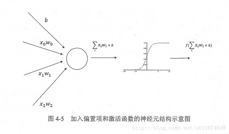
常用的激活函数有:
这里写图片描述

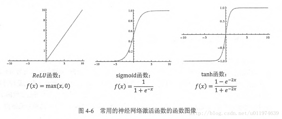
针对上面讲的神经网络，这里我们加入偏置项和激活函数的神经网络结构如下:
这里写图片描述

新的神经网络模型前向传播算法的计算办法为:
这里写图片描述

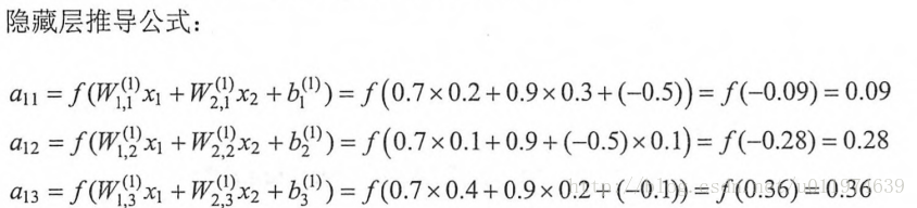
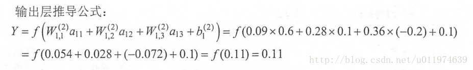
多层

多层神经网络有组合特征提取的功能，这个特性对解决不易提取特征向量的问题有很大帮助.这也是深度学习在多种问题上突破的原因.

损失函数

神经网络模型的效果以及优化目标是通过损失函数(loss function)来定义的.

经典损失函数

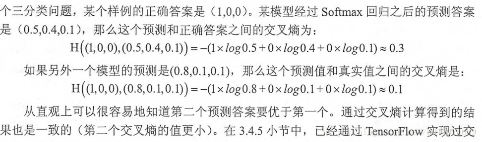
分类问题和回归问题是监督学习的两大种类。在分类问题上，通过神经网络解决分类问题常用的方法是设置n个输出节点，n为类别的个数。这时候需要判断输出指标，该如何确定一个输出向量和期望的向量有多接近。这里我们使用了交叉熵损失函数。

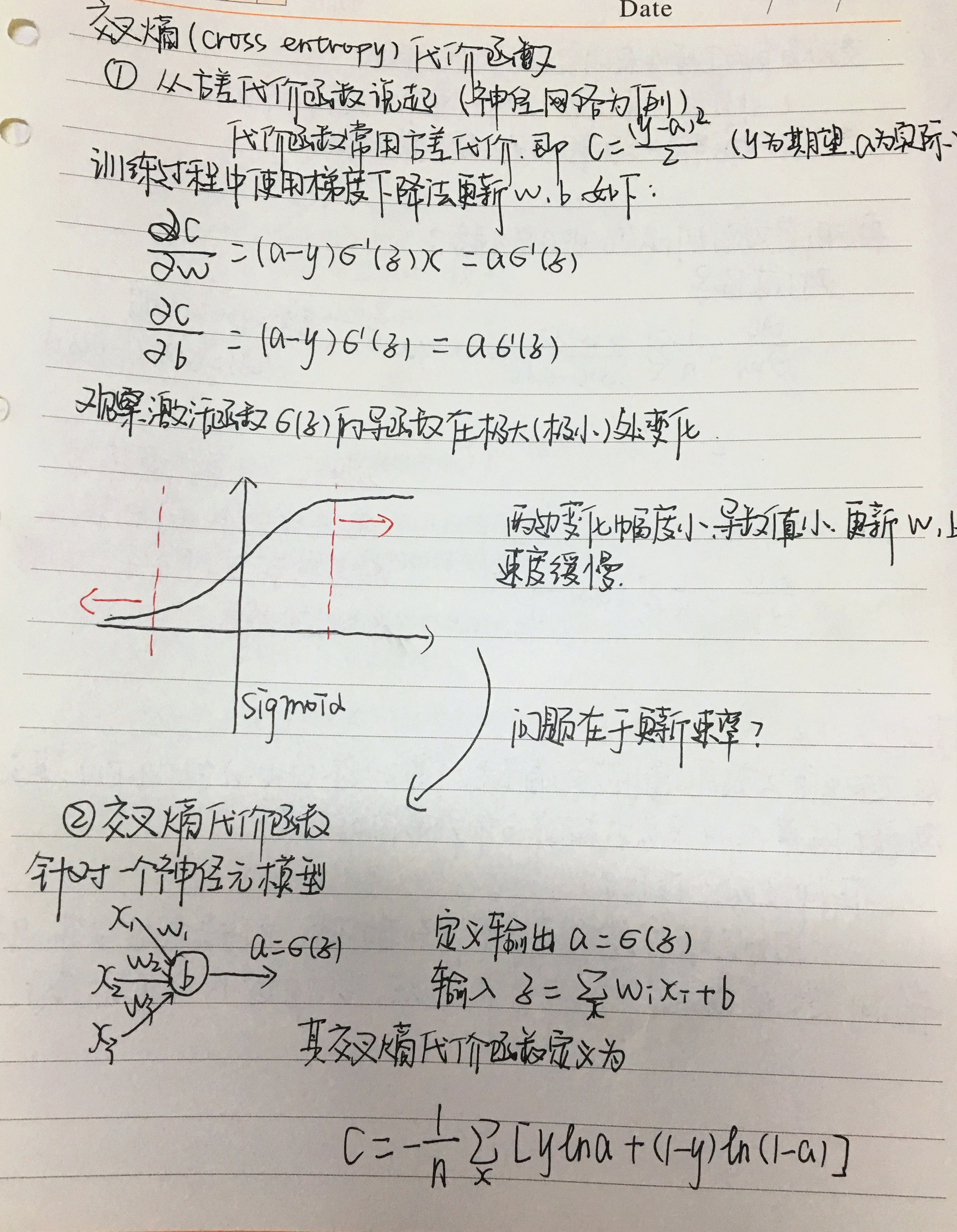
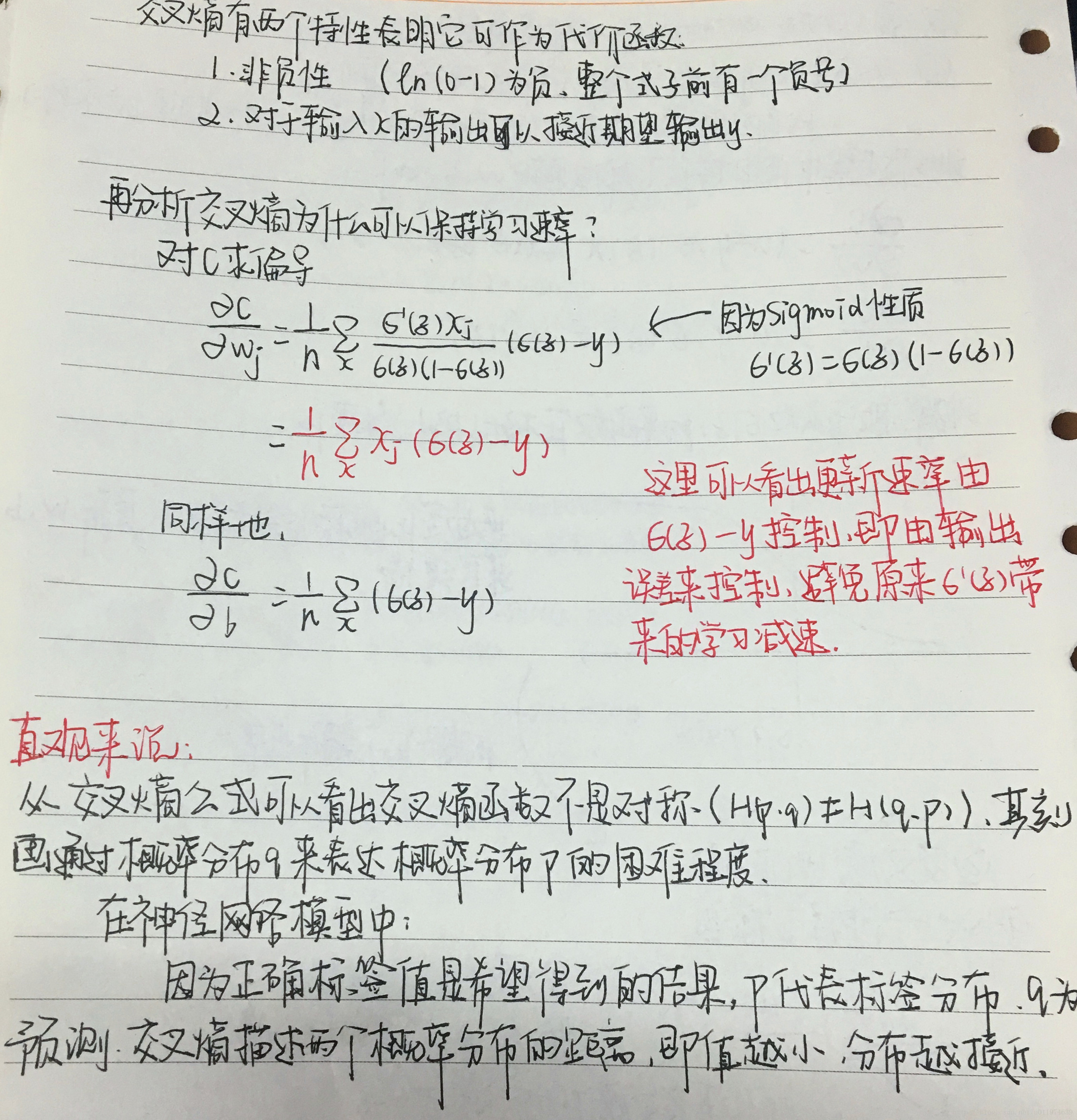
交叉熵

交叉熵(cross entropy)是分类问题常用的评判方法之一.

熵熵的本质是香农信息量的期望。

这里写图片描述

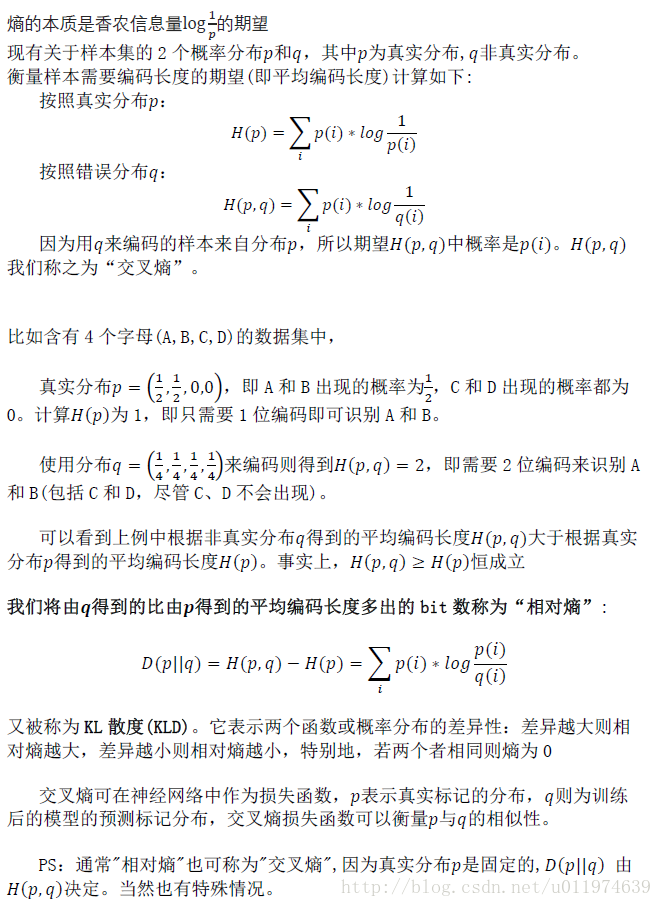
分类问题-交叉熵

交叉熵刻画的是通过两个概率分布的距离，即通过概率分布q表达概率分布p的困难程度
这里写图片描述

给出一个具体的样例直观的说明交叉熵可以判断预测与标签值之间的距离:
这里写图片描述

TensorFlow中的交叉熵实现

我们实现的交叉熵代码如下:

cross_entropy = -tf.reduce_mean(y_ * tf.log(tf.clip_by_value(y, 1e-10, 1.0)))
其中y_代表标签值，y代表预测值。
 
 1
2

先说tf.clip_by_value函数，该函数可以将一个张量的值限制在一个范围内

    v = tf.constant([[1.0,2.0,3.0],[4.0,5.0,6.0]])
    print tf.clip_by_value(v,2.5,4.5).eval()
    #v中小于2.5的转换为2.5 大约4.5的转换为4.5

    tf.clip_by_value(y,1e-10,1.0)
    #保证下一步的log值不会错误

tf.log 即完成对张量中所有元素的依次求对数功能

    v = tf.constant([1.0,2.0,3.0])
    print tf.log(v).eval()
    #输出[ 0.        ,  0.69314718,  1.09861231]

    tf.log(tf.clip_by_value(y, 1e-10, 1.0))
    #对输出值y取对数

乘法在实现交叉熵代码中直接将两个矩阵通过*操作，代表是元素之间相乘(矩阵乘法使用的是tf.matmul函数)

    v1 = tf.constant([[1.0,2.0],[3.0,4.0]])
    v2 = tf.constant([[5.0,6.0],[7.0,8.0]])
    print (v1*v2).eval()
    #输出[[  5.  12.]  [ 21.  32.]]

    print tf.matmul(v1,v2).eval()
    #输出[[ 19.  22.] [ 43.  50.]]

    y_ * tf.log(tf.clip_by_value(y, 1e-10, 1.0))
    #完成了对于每一个样例中的每一个类别交叉熵p(x)logq(x)的计算.
    #得到一个n × m的矩阵,n为一个batch数量，m为分类类别的数量。

取平均值根据交叉熵公式，应该将每行中m个结果相加得到所有样例的交叉熵，再对n行取平均得到一个batch的平均交叉熵.因为分类问题的类别数量不变，可以直接对整个矩阵平均.
```
    v = tf.constant([[1.0,2.0,3.0],[4.0,5.0,6.0]])
    print tf.reduce_mean(v).eval()
    #平均输出为3.5

    -tf.reduce_mean(y_ * tf.log(tf.clip_by_value(y, 1e-10, 1.0)))
```

因为交叉熵一般会与Softmax回归一起使用,所以TensorFlow对这两个功能统一封装，并提供
tf.nn.softmax_cross_entropy_with_logits函数.使用下面程序实现softmax回归后的交叉熵损失函数:

cross_entropy = tf.nn.softmax_cross_entropy_with_logits(y,y_)

在只有一个正确答案的分类问题中，TensorFlow提供了tf.nn.sparse_softmax_cross_entropy_with_logits()函数进一步加速计算过程。

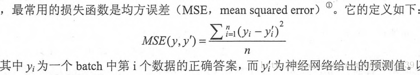
回归问题-均方误差(MSE,mean squared error)

回归问题解决的是对具体数值的预测，需要预测的不是一个事先定义好的类别，而是一个任意实数。解决回归问题的神经网络一般只有一个输出节点，这个节点的输出值就是预测值.
这里写图片描述
使用TensorFlow代码表示如下:

mse = tf.reduce_mean(tf.square(y_-y))
 
 1

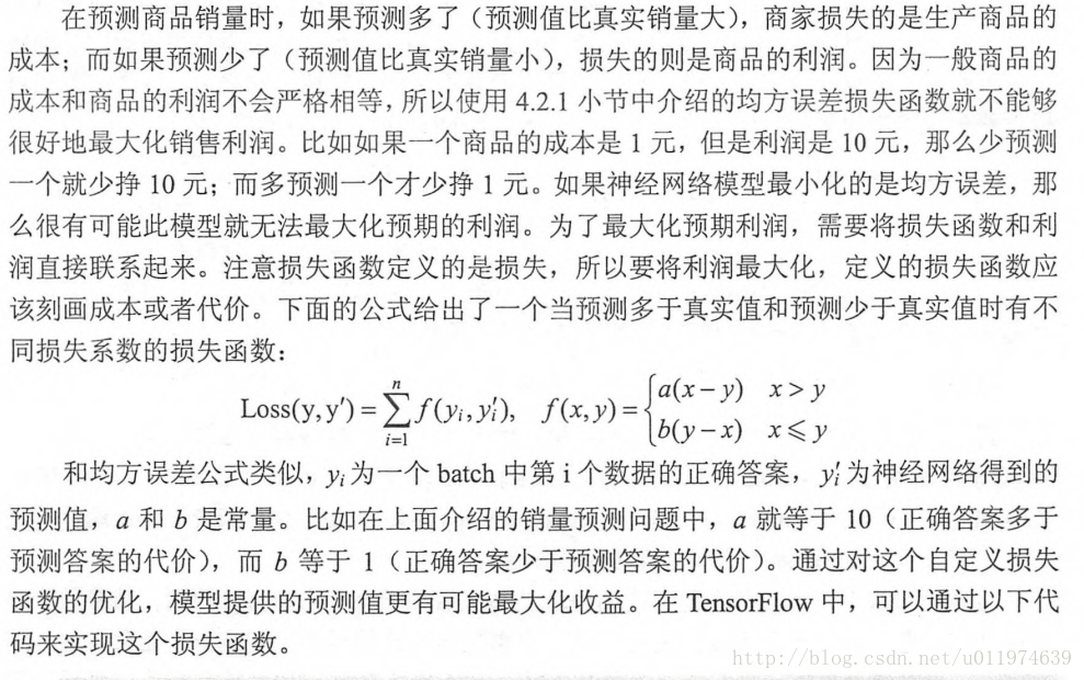
自定义损失函数

TensorFlow支持自定义损失函数。例如
这里写图片描述

loss = tf.reduce_sum(tf.select(tf.greater(v1,v2),(v1-v2)*a,(v2-v1)*b))
 
 1

在此段代码中用了两个函数

比较函数 tf.greater(v1,v2)
tf.greater(v1,v2)的输入是两个张量，函数会比较两个张量每一个元素的大小，返回操作结果

选择条件函数 tf.select(select不可用，暂时不知道原因)
tf.select有三个参数，第一个是选择条件的根据(类似?:操作符)，如果为True则选中第二个参数.否则选中第三个参数

#  coding:utf8
import tensorflow as tf

v1 = tf.constant([1.0, 2.0, 3.0, 4.0])
v2 = tf.constant([4.0, 3.0, 2.0, 1.0])

with tf.Session() as sess:
    print(sess.run(tf.greater(v1, v2)))
    print(sess.run(tf.where(tf.greater(v1, v2), v1, v2))) 
    #select不可用，使用where代替

输出:
[False False  True  True]
[4.0 3.0 3.0 4.0]

使用自定义函数的完整历程代码:

    #  coding:utf8

    import tensorflow as tf

    #使用NumPy工具包生成模拟数据集
    from numpy.random import RandomState

    #定义训练数据batch大小
    batch_size = 8


    #输出一般只有一个输出节点
    x = tf.placeholder(tf.float32, shape=(None, 2), name='x-input')
    y_ = tf.placeholder(tf.float32, shape=(None, 1), name='y-input')

    #定义一个单层神经网络前向传播过程,这里就是简单的加权和
    w1 = tf.Variable(tf.random_normal([2, 1], stddev=1, seed=1))
    y = tf.matmul(x, w1)


    #定义预测成本
    loss_less = 10
    loss_more = 1
    loss = tf.reduce_sum(tf.where(tf.greater(y,y_),(y-y_)*loss_more,(y_-y)*loss_less))

    # 定义学习率
    learning_rate = 0.001

    # 定义BP算法优化神经网络参数
    train_step = tf.train.AdamOptimizer(learning_rate).minimize(loss)

    #通过随机数生成一个数据集
    rdm = RandomState(1)
    dataset_size = 128
    X = rdm.rand(dataset_size,2)

    #设置回归的正确值为两个输入的和加上一个噪声值。
    Y = [[x1+x2+rdm.rand()/10.0-0.05] for (x1,x2) in X]

    #创建会话运行程序
    with tf.Session() as sess:
        sess.run(tf.initialize_all_variables())

        STEPS = 5000
        for i in range(STEPS):
            #每次选取batch_size个样本训练
            start = (i*batch_size) % dataset_size
            end = min(start+batch_size,dataset_size)
            sess.run(train_step,feed_dict={x:X[start:end], y_:Y[start:end]})
        print(sess.run(w1))


输出

    [[ 1.01934707]
    [ 1.04280913]]
 
 1
2
3
4
5
6
7
8
9
10
11
12
13
14
15
16
17
18
19
20
21
22
23
24
25
26
27
28
29
30
31
32
33
34
35
36
37
38
39
40
41
42
43
44
45
46
47
48
49
50
51
52
53
54
55
56

神经网络优化算法

本节更加具体的介绍如何通过BP算法和梯度下降法调整神经网络的参数。梯度下降法主要用于优化单个参数的取值，而BP算法给出了一个高效的方式在所有参数上使用梯度下降法，从而使神经网络在训练数据上损失函数尽可能的小.
这里写图片描述

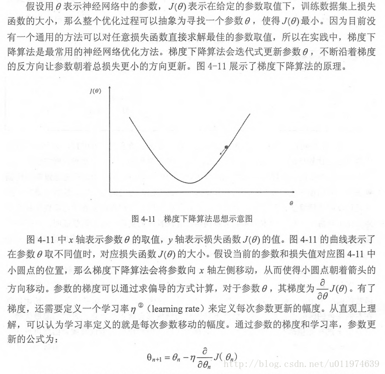
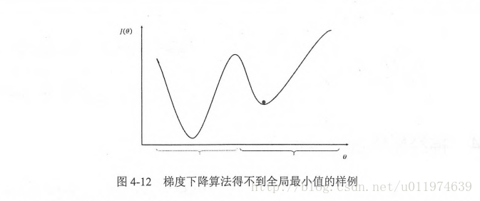
需要注意的是，梯度下降法并不能保证被优化的函数达到全局最优解。
图示，优化点陷入局部最优解，而不是全局最优。可见在训练神经网络时，参数的初始值会很大程度影响最后得到的结果.
这里写图片描述

梯度下降法的计算时间太长。因为要在全部的训练数据上最小化损失，所以损失函数J(θ)是所有训练数据的损失和。在海量数据下，计算全部训练数据上的损失函数是非常耗时的。

为了加速训练过程，可以使用随机梯度下降法(stochastic gradient descent)。这个算法是在每一轮迭代中，随机优化某一条训练数据上的损失函数。这样速度就大大加快了。同时这方法的问题也很明显:使用随机梯度下降法可能连局部最优也达不到。

这里采用折中的办法:每次计算一小部分训练数据的损失函数(即一个batch)，通过矩阵运算。每次一个batch上优化神经网络参数速度并不会太慢，这样收敛速度得到的保证，收敛结果也接近梯度下降的效果。

下面代码给出了TensorFlow中如何实现神经网络的大致训练过程:

#定义训练数据batch大小
    batch_size = n


    #每次读取一小部分
    x = tf.placeholder(tf.float32,shape=(batch_size,2),name='x-input')
    y_ = tf.placeholder(tf.float32,shape=(batch_size,1),name='y-input')


    #定义神经网络结构和优化算法
    loss =...

    # 定义学习率
    learning_rate = 0.001

    # 定义BP算法优化神经网络参数
    train_step = tf.train.AdamOptimizer(learning_rate).minimize(loss)

    #训练网络
    with tf.Session() as sess:
        #参数初始化等
        sess.run(tf.initialize_all_variables())

        #迭代更新参数
        STEPS = 5000
        for i in range(STEPS):
            #每次选取batch_size个样本训练,一般将所有训练数据打乱后选取
            current_X,current_Y = ...
            sess.run(train_step,feed_dict={x:X[start:end], y_:Y[start:end]})
 
 1
2
3
4
5
6
7
8
9
10
11
12
13
14
15
16
17
18
19
20
21
22
23
24
25
26
27
28
29

学习率的设置

学习率决定参数每次更新的幅度，如果幅度过大，可能导致参数在最优值两侧来回移动。如果幅度过小，会大大降低优化速度。为了解决这个问题，TensorFlow提供了一种更加灵活的学习率设置方法–指数衰减法。使用以下函数

tf.train.exponential_decay(
    learning_rate,
    global_step,
    decay_steps,
    decay_rate,
    staircase=False,
    name=None
)

参数含义:

learning_rate: A scalar float32 or float64 Tensor or a Python number. The initial learning rate.(初始学习率)
global_step: A scalar int32 or int64 Tensor or a Python number. Global step to use for the decay computation. Must not be negative.
decay_steps: A scalar int32 or int64 Tensor or a Python number. Must be positive. See the decay computation above.(衰减速度)
decay_rate: A scalar float32 or float64 Tensor or a Python number. The decay rate.(衰减系数)
staircase: Boolean. If True decay the learning rate at discrete intervals
name: String. Optional name of the operation. Defaults to ‘ExponentialDecay’.

函数功能:
The function returns the decayed learning rate. It is computed as:

decayed_learning_rate = learning_rate *
                    decay_rate ^ (global_step / decay_steps)

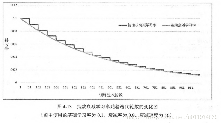
如果参数staircase为True，global_step / decay_steps 结果会取整，此时学习率成为阶梯函数(staircase function).
下图连续的学习率曲线是staircase为False，阶梯曲线是staircase为True.
这里写图片描述

应用示例:
Example: decay every 100000 steps with a base of 0.96:

global_step = tf.Variable(0, trainable=False)
    starter_learning_rate = 0.1
    learning_rate = tf.train.exponential_decay(starter_learning_rate, global_step,
                                               100000, 0.96, staircase=True)
    # Passing global_step to minimize() will increment it at each step.
    learning_step = (
        tf.train.GradientDescentOptimizer(learning_rate)
        .minimize(...my loss..., global_step=global_step)
 
 1
2
3
4
5
6
7
8

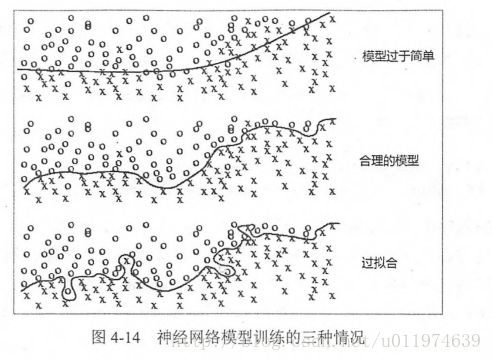
过拟合问题

过度拟合训练数据中的随机噪声虽然可以得到非常小的损失函数，但是对未知数据可能无法做出可靠的判断.如下图:
这里写图片描述

使用TensorFlow可以优化任意形式的损失函数，以下代码给出了一个简单的带L2正则化的损失函数定义:

#tensorflow.contrib.layers模块需要导入
    import  tensorflow.contrib.layers as tflayers

    w = tf.Variable(tf.random_normal([2,1],stddev=1,seed=1))
    y = tf.matmul(x,w)

    loss = tf.reduce_mean(tf.square(y_ - y)) +                    tflayers.l2_regularizer(lambda)(w)  
    #lambda为正则化权重  实际过程中lambda为关键字
 
 1
2
3
4
5
6
7
8

loss定义为损失函数，由两个部分组成，第一个部分是均方误差损失函数，刻画模型在训练数据上的表现。第二部分就是正则化，防止模型过度模拟训练数据中的随机噪声.

类似的,tensorflow.contrib.layers.l1_regularizer可以计算L1正则化的值。

在简单的神经网络中，上述代码可以很好地计算带正则化的损失函数，但当神经网络的参数增多之后，这样的方式可能导致loss函数定义可读性变差，更主要的是导致，网络结构复杂之后定义网络结构的部分和计算损失函数的部分可能不在同一函数中，这样通过变量这样方式计算损失函数就不方便了.

以下代码使用TensorFlow中给提供的集合(Collection)解决一个5层神经网络带L2正则化的损失函数计算方法:

# coding=utf-8
    # tensorflow中集合的运用:损失集合
    # 计算一个5层神经网络带L2正则化的损失函数
    import tensorflow as tf
    import  tensorflow.contrib.layers as tflayers
    from numpy.random import RandomState

    #获得一层神经网络边上的权重，并将这个权重的L2 正则化损失加入名称为'losses'的集合里
    def get_weight(shape, lamada):
        # 生成对应一层的权重变量
        var = tf.Variable(tf.random_normal(shape), dtype=tf.float32)
        tf.add_to_collection('losses', tflayers.l2_regularizer(lamada)(var))
        return var

    x = tf.placeholder(tf.float32, shape=(None, 2), name='x_input')
    y_ = tf.placeholder(tf.float32, shape=(None, 1), name='y_input')

    batch_size = 8

    # 定义每层神经网络的节点个数
    layer_dimension = [2, 10, 10, 10, 1]
    # 获取神经网络的层数
    n_layers = len(layer_dimension)
    # 这个变量表示前向传播时最深层的节点，最开始的时候是输入层
    cur_layer = x
    # 当前层的节点个数
    in_dimension = layer_dimension[0]

    # 通过一个循环生成5层全连接的神经网络结构
    for i in range(1, n_layers):
        # 获取下一层节点的个数
        out_dimension = layer_dimension[i]
        # 获取当前计算层的权重并加入了l2正则化损失
        weight = get_weight([in_dimension, out_dimension], 0.001)
        # 随机生成偏向
        bias = tf.Variable(tf.constant(0.1, shape=[out_dimension]))
        # 计算前向传播节点，使用RELU激活函数
        cur_layer = tf.nn.relu(tf.matmul(cur_layer, weight) + bias)
        # 进入下一层之前，更新下一层节点的输入节点数
        in_dimension = layer_dimension[i]

    # 计算模型数据的均值化损失加入损失集合
    mse_loss = tf.reduce_mean(tf.square(y_ - cur_layer))
    tf.add_to_collection('losses', mse_loss)

    # get_collection返回一个列表，列表是所有这个集合的所有元素
    # 在本例中，元素代表了其他的损失，加起来就得到了所有的损失
    loss = tf.add_n(tf.get_collection('losses'))

    global_step = tf.Variable(0)
    # 学习率的设置：指数衰减法，参数：初始参数，全局步骤，每训练100轮乘以衰减速度0,96(当staircase=True的时候)
    learning_rate = tf.train.exponential_decay(0.1, global_step, 100, 0.96, staircase=True)
    train_step = tf.train.GradientDescentOptimizer(learning_rate).minimize(loss, global_step=global_step)

    rdm = RandomState(1)
    dataset_size = 128
    X = rdm.rand(dataset_size, 2)
    # 加入了一个噪音值，-0.05～0.05之间
    Y = [[x1 + x2 + rdm.rand() / 10.0 - 0.05] for (x1, x2) in X]

    with tf.Session() as sess:
        init_op = tf.initialize_all_variables()
        sess.run(init_op)
        # print sess.run(w1)

        steps = 5000
        for i in range(steps):
            start = (i * batch_size) % dataset_size
            end = min(start + batch_size, dataset_size)

            sess.run(train_step, feed_dict={x: X[start:end], y_: Y[start:end]})
            if i % 1000 == 0:
                total_loss = sess.run(
                    loss, feed_dict={x: X, y_: Y})
                print("After %d training_step(s) ,loss on all data is %g" % (i, total_loss))
                # print sess.run(w1)
 
 1
2
3
4
5
6
7
8
9
10
11
12
13
14
15
16
17
18
19
20
21
22
23
24
25
26
27
28
29
30
31
32
33
34
35
36
37
38
39
40
41
42
43
44
45
46
47
48
49
50
51
52
53
54
55
56
57
58
59
60
61
62
63
64
65
66
67
68
69
70
71
72
73
74
75
76

滑动平均模型

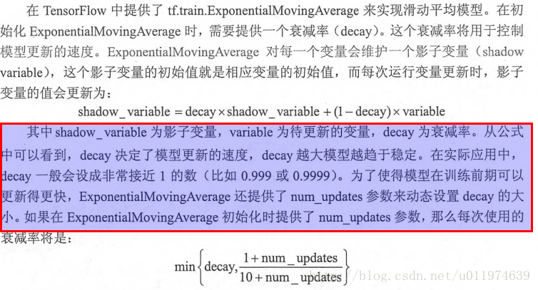
在采用随机梯度下降算法训练神经网络时，使用滑动平均算法模型可以提供模型的鲁棒性(robust).TensorFlow中提供了tf.train.ExponentialMovingAverage来实现滑动平均模型.
这里写图片描述

Maintains moving averages of variables by employing an exponential decay.

When training a model, it is often beneficial to maintain moving averages of the trained parameters. Evaluations that use averaged parameters sometimes produce significantly better results than the final trained values.

The apply() method adds shadow copies of trained variables and add ops that maintain a moving average of the trained variables in their shadow copies. It is used when building the training model. The ops that maintain moving averages are typically run after each training step. The average() and average_name() methods give access to the shadow variables and their names. They are useful when building an evaluation model, or when restoring a model from a checkpoint file. They help use the moving averages in place of the last trained values for evaluations.


通过指数衰减完成滑动平均计算，创建一个ExponentialMovingAverage对象时要指定衰减率(decay).衰减率用于控制模型更新速度。每一个变量会有一个shadow_variables，这个shadow_variables初始值就是对应变量的初始值。shadow_variables的更新公式如下:

shadow_variable -= (1 - decay) * (shadow_variable - variable)

decay设置值应该接近于1.0（ 例如0.999, 0.9999）

Example usage when creating a training model:

#coding=utf-8
    #滑动平均模型的小程序
    #滑动平均模型可以使得模型在测试数据上更加健壮
    import tensorflow as tf

    #定义一个变量用以计算滑动平均，变量的初始值为0,手动指定类型为float32，
    #因为所有需要计算滑动平均的变量必须是实数型
    v1 = tf.Variable(0,dtype=tf.float32)

    #模拟神经网络迭代的轮数，动态控制衰减率
    step = tf.Variable(0,trainable=False)
    #定义一个滑动平均的类，初始化时给定衰减率为0.99和控制衰减率的变量
    ema = tf.train.ExponentialMovingAverage(0.99,step)

    #定义一个滑动平均的操作，这里需要给定一个列表，每次执行这个操作时，列表里的元素都会被更新
    maintain_average_op = ema.apply([v1])

    with tf.Session() as sess:
        #初始化所有变量
        init_op = tf.initialize_all_variables()
        sess.run(init_op)

        #获取滑动平均之后变量的取值
        print sess.run([v1,ema.average(v1)])

        #更新v1的值为5
        sess.run(tf.assign(v1,5))
        #更新v1的滑动平均值，衰减率为min{0.99,(1+step)/(10+step)=0.1}=0.1,
        #所以v1的滑动平均被更新为0.1*0+0.9*5=4.5
        sess.run(maintain_average_op)
        print sess.run([v1,ema.average(v1)])

        #更新迭代的轮数
        sess.run(tf.assign(step,10000))
        sess.run(tf.assign(v1,10))
        #这里的衰减率变成0.99
        #v1 = 0.99*4.5+0.01*10=4.555
        sess.run(maintain_average_op)
        print sess.run([v1,ema.average(v1)])

        #再次更新滑动平均值
        sess.run(maintain_average_op)
        print sess.run([v1,ema.average(v1)])

输出

    [0.0, 0.0]
    [5.0, 4.5]
    [10.0, 4.5549998]
    [10.0, 4.6094499]
 
 1
2
3
4
5
6
7
8
9
10
11
12
13
14
15
16
17
18
19
20
21
22
23
24
25
26
27
28
29
30
31
32
33
34
35
36
37
38
39
40
41
42
43
44
45
46
47
48
49
50

TensorFlow实现Softmax Regression 识别手写数字

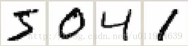
MNIST(Mixed National Institute of Standards and Technology database)是一个非常有名的机器视觉数据集，由几万张28x28像素的手写数字组成，这些图片只包含灰度值。我们的任务就是对这些图片分成数字0~9类。
这里写图片描述

下载和加载数据：

    from tensorflow.examples.tutorials.mnist import input_data
    mnist = input_data.read_data_sets('MNIST_data/',one_hot=True)

    #download...
    Extracting MNIST_data/train-images-idx3-ubyte.gz
    Extracting MNIST_data/train-labels-idx1-ubyte.gz
    Extracting MNIST_data/t10k-images-idx3-ubyte.gz
    Extracting MNIST_data/t10k-labels-idx1-ubyte.gz
 
 1
2
3
4
5
6
7
8

查看数据集：

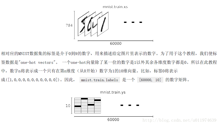
在MNIST数据集中，mnist.train.images是一个形状为[60000,784]的张量，第一个维度数字用来索引图片，第二个维度数字用来索引每张图片中的像素点。在此张量里的每一个元素，都表示某张图片里的某个像素的强度值，值介于0和1之间。
这里写图片描述

训练集

 >>> print(mnist.train.images.shape,mnist.train.labels.shape)
        ((55000, 784), (55000, 10))
 
 1
2

其中训练集有55000个样本，是一个55000x784的Tensor.第一个维度是图片的编号，第二个维度是图片中像素点的编号。

训练集的Label是一个55000x10的Tensor，对10个种类的one-hot编码，即对应n位为1代表数值为n.

类似的测试集和校验集一样

测试集和校验集

    print(mnist.test.images.shape,mnist.test.labels.shape)
    ((10000, 784), (10000, 10))
    >>> print(mnist.validation.images.shape,mnist.validation.labels.shape)
    ((5000, 784), (5000, 10))
 
 1
2
3
4

选取数据

input_data.read_data_sets函数生成的类提供了mnist.train.next_batch函数，可以从所有的训练数据中读取一小部分作为一个训练batch.

    from tensorflow.examples.tutorials.mnist import input_data
    mnist = input_data.read_data_sets('/path/to/MNIST_data',one_hot=True)

    batch_size = 100
    xs,ys = mnist.train.next_batch(batch_size)
    print xs.shape
    >>> (100, 784)
    print ys.shape
    >>> (100, 10)
 
 1
2
3
4
5
6
7
8
9

设计算法

Softmax Regression简介

处理多分类任务时，通常使用Softmax Regression模型。
在神经网络中，如果问题是分类模型(即使是CNN或者RNN)，一般最后一层是Softmax Regression。
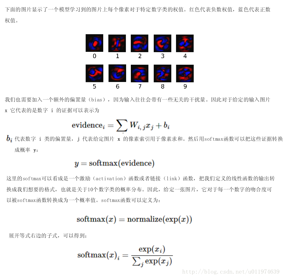
它的工作原理是将可以判定为某类的特征相加，然后将这些特征转化为判定是这一类的概率。
这里写图片描述

这里写图片描述

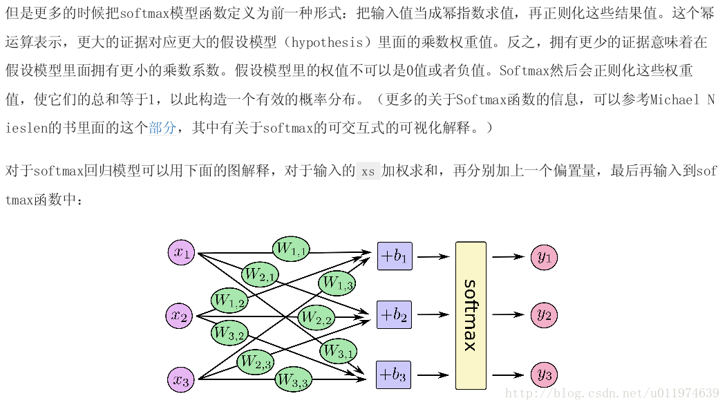
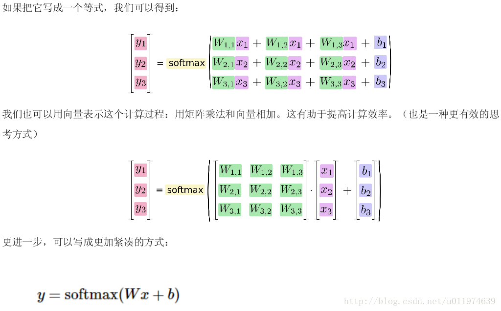
实现Softmax Regression

创建一个神经网络模型步骤如下:

定义网络结构(即网络前向算法)
定义loss function，确定Optimizer
迭代训练
在测试集/验证集上测评

1. 定义网络结构

    import tensorflow as tf

    sess = tf.InteractiveSession() #注册默认Session

    #输入数据占位符,None代表输入条数不限制(取决训练的batch_size)
    x = tf.placeholder("float", [None, 784]) 

    W = tf.Variable(tf.zeros([784,10])) #权重张量，weights无隐藏层
    b = tf.Variable(tf.zeros([10])) #偏置biases

    #实现softmax Regression  y=softmax(Wx+b)
    y = tf.nn.softmax(tf.matmul(x,W) + b) 
 
 1
2
3
4
5
6
7
8
9
10
11
12

2. 定义loss function，确定Optimizer

    #y_为标签值
    y_ = tf.placeholder("float", [None,10])

    #交叉熵损失函数定义
    cross_entropy = -tf.reduce_mean(tf.reduce_sum(y_*tf.log(y)))

    #学习率定义
    learn_rate = 0.001

    #优化器选择
    train_step = tf.train.GradientDescentOptimizer(learn_rate).minimize(cross_entropy)
 
 1
2
3
4
5
6
7
8
9
10
11

3. 迭代训练

with Session() as sess:
        #初始化所有变量
        init_op = tf.global_variables_initializer()
        sess.run(init_op)

        #迭代次数
        STEPS = 1000
        for i in range(STEPS):
            #使用mnist.train.next_batch随机选取batch
            batch_xs, batch_ys = mnist.train.next_batch(100)
            sess.run(train_step, feed_dict={x: batch_xs, y_: batch_ys})
 
 1
2
3
4
5
6
7
8
9
10
11

4. 在测试集/验证集上测评

#tf.argmax函数可以在一个张量里沿着某条轴的最高条目的索引值
    #tf.argmax(y,1) 是模型认为每个输入最有可能对应的那些标签
    #而 tf.argmax(y_,1) 代表正确的标签
    #我们可以用 tf.equal 来检测我们的预测是否真实标签匹配
    correct_prediction = tf.equal(tf.argmax(y,1), tf.argmax(y_,1))
    #这行代码会给我们一组布尔值。


    #为了确定正确预测项的比例,我们可以把布尔值转换成浮点数,然后取平均值。例如, [True, False, True, True] 会变成 [1,0,1,1] ,取平均值后得到 0.75
    accuracy = tf.reduce_mean(tf.cast(correct_prediction, tf.float32))

    #我们计算所学习到的模型在测试数据集上面的正确率
    print sess.run(accuracy, feed_dict={x: mnist.test.images, y_: mnist.test.labels})
 
 1
2
3
4
5
6
7
8
9
10
11
12
13

下面给出一个完整的TensorFlow训练神经网络

这里会用到激活函数去线性化，使用更深层网络，使用带指数衰减的学习率设置，同时使用正则化避免过拟合，以及使用滑动平均模型来使最终模型更加健壮。

# coding=utf-8
    # 在MNIST 数据集上实现神经网络
    # 包含一个隐层
    # 5种优化方案：激活函数，多层隐层，指数衰减的学习率，正则化损失，滑动平均模型

    import tensorflow as tf
    import tensorflow.contrib.layers as tflayers
    from tensorflow.examples.tutorials.mnist import input_data


    #MNIST数据集相关参数
    INPUT_NODE = 784  #输入节点数
    OUTPUT_NODE = 10 #输出节点数

    LAYER1_NODE = 500 #选择一个隐藏层,节点数为500
    BATCH_SIZE = 100 #一个batch大小


    '''
    指数衰减学习率
    函数定义exponential_decay(learning_rate, global_step, decay_steps, decay_rate, staircase=False, name=None):
        计算公式:decayed_learning_rate = learning_rate * decay_rate ^ (global_step / decay_steps)
            learning_rate = LEARNING_RATE_BASE;   
            decay_rate = LEARNING_RATE_DECAY
            global_step=TRAINING_STEPS;
            decay_steps = mnist.train.num_examples/batch_size
    '''
    LEARNING_RATE_BASE = 0.8  # 基础的学习率，使用指数衰减设置学习率
    LEARNING_RATE_DECAY = 0.99  # 学习率的初始衰减率


    # 正则化损失的系数
    LAMADA = 0.0001
    # 训练轮数
    TRAINING_STEPS = 30000
    # 滑动平均衰减率
    MOVING_AVERAGE_DECAY = 0.99




    def get_weight(shape, llamada):
        '''
        function:生成权重变量，并加入L2正则化损失到losses集合里

        :param shape:   权重张量维度
        :param llamada: 正则参数
        :return:    权重张量(所有权重都添加在losses集合中,简化计算loss操作)

        tf.truncated_normal(shape, mean=0.0, stddev=1.0, dtype=tf.float32, seed=None, name=None)
        从截断的正态分布中输出随机值
        生成的值服从具有指定平均值和标准偏差的正态分布，如果生成的值大于平均值2个标准偏差的值则丢弃重新选择。
            :shape: 一维的张量，也是输出的张量
            :mean: 正态分布的均值。
            :stddev: 正态分布的标准差。
            :dtype: 输出的类型。
            :seed: 一个整数，当设置之后，每次生成的随机数都一样。
            :name: 操作的名字。

        '''
        weights = tf.Variable(tf.truncated_normal(shape, stddev=0.1))
        if llamada != None:
            tf.add_to_collection('losses', tflayers.l2_regularizer(llamada)(weights))
        return weights


    def inference(input_tensor, avg_class, weights1, biases1, weights2, biases2):
        '''
        对神经网络进行前向计算，如果avg_class为空计算普通的前向传播，否则计算包含滑动平均的前向传播
        使用了RELU激活函数实现了去线性化
        :param input_tensor: 输入张量
        :param avg_class:   平均滑动类
        :param weights1:    一级层权重
        :param biases1:     一级层偏置
        :param weights2:    二级层权重
        :param biases2:     二级层权重
        :return:    前向传播的计算结果(默认隐藏层一层,所以输出层没有ReLU)

        计算输出层的前向传播结果。
        因为在计算损失函数的时候会一并计算softmax函数，因此这里不加入softmax函数
        同时，这里不加入softmax层不会影响最后的结果。
        因为，预测时使用的是不同类别对应节点输出值的相对大小，因此有无softmax层对最后的结果没有影响。
        '''
        if avg_class == None:
            layer1 = tf.nn.relu(tf.matmul(input_tensor, weights1) + biases1)
            return tf.matmul(layer1, weights2) + biases2
        else:
            # 首先需要使用avg_class.average函数计算变量的滑动平均值，然后再计算相应的神经网络前向传播结果
            layer1 = tf.nn.relu(
                tf.matmul(input_tensor, avg_class.average(weights1)) + avg_class.average(biases1))
            return tf.matmul(layer1, avg_class.average(weights2)) + avg_class.average(biases2)


    # 训练模型的过程
    def train(mnist):
        '''
        训练函数过程:
            1.定义网络结构,计算前向传播结果
            2.定义loss和优化器
            3.迭代训练
            4.评估训练模型

        :param mnist: 数据集合
        :return:
        '''

        x = tf.placeholder(tf.float32, shape=(None, INPUT_NODE), name='x_input')
        y_ = tf.placeholder(tf.float32, shape=(None, OUTPUT_NODE), name='y_input')

        # 生成隐藏层(使用get_weight带L2正则化)
        weights1 = get_weight([INPUT_NODE, LAYER1_NODE], LAMADA)
        biaes1 = tf.Variable(tf.constant(0.1, shape=[LAYER1_NODE]))
        # 生成输出层的参数
        weights2 = get_weight([LAYER1_NODE, OUTPUT_NODE], LAMADA)
        biaes2 = tf.Variable(tf.constant(0.1, shape=[OUTPUT_NODE]))
        # 计算神经网络的前向传播结果，注意滑动平均的类函数为None
        y = inference(x, None, weights1, biaes1, weights2, biaes2)
        # 定义存储模型训练轮数的变量，并指明为不可训练的参数
        global_step = tf.Variable(0, trainable=False)

        '''
        使用平均滑动模型
            1.初始化滑动平均的函数类，加入训练轮数的变量可以加快需年早期变量的更新速度
            2.对神经网络里所有可训练参数（列表）应用滑动平均模型，每次进行这个操作，列表里的元素都会得到更新
            3.计算使用了滑动平均的网络前向传播结果，滑动是维护影子变量来记录其滑动平均值,需要使用时要明确调用average函数
        '''
        variable_averages = tf.train.ExponentialMovingAverage(MOVING_AVERAGE_DECAY, global_step)
        variable_averages_op = variable_averages.apply(tf.trainable_variables())
        average_y = inference(x, variable_averages, weights1, biaes1, weights2, biaes2)

        '''
        定义loss
            当只有一个标准答案的时候，使用sprase_softmax_cross_entropy_with_logits计算损失，可以加速计算
                参数：不包含softma层的前向传播结果，训练数据的正确答案
                因为标准答案是一个长度为10的一维数组，而该函数需要提供一个正确答案的数字
                因此需要使用tf.argmax函数得到正确答案的对应类别编号
        '''
        cross_entropy = tf.nn.sparse_softmax_cross_entropy_with_logits(logits=y, labels=tf.argmax(y_, 1))
        # 计算在当前batch里所有样例的交叉熵平均值，并加入损失集合
        cross_entropy_mean = tf.reduce_mean(cross_entropy)
        tf.add_to_collection('losses', cross_entropy_mean)
        # get_collection返回一个列表，列表是所有这个集合的所有元素(在本例中，元素代表了其他部分的损失，加起来就得到了所有的损失)
        loss = tf.add_n(tf.get_collection('losses'))

        '''
        设置指数衰减的学习率
            使用GradientDescentOptimizer()优化算法的损失函数
        '''
        learning_rate = tf.train.exponential_decay(LEARNING_RATE_BASE,  # 基础的学习率，在此基础上进行递减
                                                   global_step,  # 迭代的轮数
                                                   mnist.train.num_examples / BATCH_SIZE,  # 所有的数据得到训练所需要的轮数
                                                   LEARNING_RATE_DECAY)  # 学习率衰减速度
        train_step = tf.train.GradientDescentOptimizer(learning_rate).minimize(loss, global_step=global_step)


        '''
        在训练神经网络模型的时候，每过一次数据既需要BP更新参数又要更新参数的滑动平均值。
        为了一次完成多种操作，tensroflow提供了两种机制:tf.control_dependencies和tf.group

        下面的两行程序和：train_op = tf.group(train_step,variables_average_op)等价

        tf.group(*inputs, **kwargs )
            Create an op that groups multiple operations.
            When this op finishes, all ops in input have finished. This op has no output.


        control_dependencies(control_inputs)
            Use with the with keyword to specify that all operations constructed within 
            the context should have control dependencies on control_inputs. 
        For example:
            with g.control_dependencies([a, b, c]):
             # `d` and `e` will only run after `a`, `b`, and `c` have executed.
              d = ...
              e = ...

        '''
        with tf.control_dependencies([train_step, variable_averages_op]):
            train_op = tf.no_op(name='train')

        '''
            进行验证集上的准确率计算，这时需要使用滑动平均模型
            判断两个张量的每一维是否相等，如果相等就返回True,否则返回False
            这个运算先将布尔型的数值转为实数型，然后计算平均值，平均值就是准确率
        '''
        correct_prediction = tf.equal(tf.argmax(average_y, 1), tf.argmax(y_, 1))
        accuracy = tf.reduce_mean(tf.cast(correct_prediction, tf.float32))




        with tf.Session() as sess:
            # init_op = tf.global_variables_initializer()  sess.run(init_op) 这种写法可视化更加清晰
            tf.global_variables_initializer().run()
            # 准备验证数据，一般在神经网络的训练过程中会通过验证数据来判断大致停止的条件和评判训练的效果
            validate_feed = {x: mnist.validation.images, y_: mnist.validation.labels}
            # 准备测试数据，在实际中，这部分数据在训练时是不可见的，这个数据只是作为模型优劣的最后评价标准
            test_feed = {x: mnist.test.images, y_: mnist.test.labels}
            # 迭代的训练神经网络
            for i in range(TRAINING_STEPS):
                xs, ys = mnist.train.next_batch(BATCH_SIZE)
                _, loss_value, step = sess.run([train_op, loss, global_step], feed_dict={x: xs, y_: ys})
                if i % 1000 == 0:
                    print("After %d training step(s), loss on training batch is %g." % (step, loss_value))

                    validate_acc = sess.run(accuracy, feed_dict=validate_feed)
                    print "After %d training step(s),validation accuracy using average model is %g " % (step, validate_acc)
                    test_acc = sess.run(accuracy, feed_dict=test_feed)
                    print("After %d training step(s) testing accuracy using average model is %g" % (step, test_acc))


    #TensorFlow主程序入口
    def main(argv=None):
        mnist = input_data.read_data_sets("MNIST_data/", one_hot=True)
        train(mnist)


    #TensorFlow提供了一个主程序入口,tf.app.run会调用上面定义的main函数
    if __name__ == '__main__':
        tf.app.run()
 
 1
2
3
4
5
6
7
8
9
10
11
12
13
14
15
16
17
18
19
20
21
22
23
24
25
26
27
28
29
30
31
32
33
34
35
36
37
38
39
40
41
42
43
44
45
46
47
48
49
50
51
52
53
54
55
56
57
58
59
60
61
62
63
64
65
66
67
68
69
70
71
72
73
74
75
76
77
78
79
80
81
82
83
84
85
86
87
88
89
90
91
92
93
94
95
96
97
98
99
100
101
102
103
104
105
106
107
108
109
110
111
112
113
114
115
116
117
118
119
120
121
122
123
124
125
126
127
128
129
130
131
132
133
134
135
136
137
138
139
140
141
142
143
144
145
146
147
148
149
150
151
152
153
154
155
156
157
158
159
160
161
162
163
164
165
166
167
168
169
170
171
172
173
174
175
176
177
178
179
180
181
182
183
184
185
186
187
188
189
190
191
192
193
194
195
196
197
198
199
200
201
202
203
204
205
206
207
208
209
210
211
212
213
214
215
216
217
218
219

输出

After 1 training step(s), loss on training batch is 3.30849.
    After 1 training step(s),validation accuracy using average model is 0.1098 
    After 1 training step(s) testing accuracy using average model is 0.1132
    After 1001 training step(s), loss on training batch is 0.19373.
    After 1001 training step(s),validation accuracy using average model is 0.9772 
    After 1001 training step(s) testing accuracy using average model is 0.9738
    After 2001 training step(s), loss on training batch is 0.169665.
    After 2001 training step(s),validation accuracy using average model is 0.9794 
    After 2001 training step(s) testing accuracy using average model is 0.9796
    After 3001 training step(s), loss on training batch is 0.147636.
    After 3001 training step(s),validation accuracy using average model is 0.9818 
    After 3001 training step(s) testing accuracy using average model is 0.9813
    After 4001 training step(s), loss on training batch is 0.129015.
    After 4001 training step(s),validation accuracy using average model is 0.9808 
    After 4001 training step(s) testing accuracy using average model is 0.9825
    After 5001 training step(s), loss on training batch is 0.109033.
    After 5001 training step(s),validation accuracy using average model is 0.982 
    After 5001 training step(s) testing accuracy using average model is 0.982
    After 6001 training step(s), loss on training batch is 0.108935.
    After 6001 training step(s),validation accuracy using average model is 0.9818 
    After 6001 training step(s) testing accuracy using average model is 0.982
.......
.......
.......
    After 27001 training step(s), loss on training batch is 0.0393247.
    After 27001 training step(s),validation accuracy using average model is 0.9828 
    After 27001 training step(s) testing accuracy using average model is 0.9827
    After 28001 training step(s), loss on training batch is 0.0422536.
    After 28001 training step(s),validation accuracy using average model is 0.984 
    After 28001 training step(s) testing accuracy using average model is 0.9822
    After 29001 training step(s), loss on training batch is 0.0512684.
    After 29001 training step(s),validation accuracy using average model is 0.9832 
    After 29001 training step(s) testing accuracy using average model is 0.9831


 
 1
2
3
4
5
6
7
8
9
10
11
12
13
14
15
16
17
18
19
20
21
22
23
24
25
26
27
28
29
30
31
32
33
34
35

判断模型效果

这里写图片描述

Waitfou

关注

2
点赞
踩
13

收藏

觉得还不错? 一键收藏
0
评论
tensorflow入门

本文转载自：tensorflow入门实战TensorFlow计算模型-计算图计算图的简单示例计算图的使用创建新的计算图管理计算图等资源图相关的api函数Tensorflow数据模型-张量张量结构name属性shape属性type属性TensorFlow中types相关属性在TensorFlow中有14种不同的类型见下表type的apiclass tfDT
复制链接

扫一扫