


In this post, we will learn the details of the Histogram of Oriented Gradients (HOG) feature descriptor. We will learn what is under the hood and how this descriptor is calculated internally by OpenCV, MATLAB and other packages.
This post is part of a series I am writing on Image Recognition and Object Detection.
The complete list of tutorials in this series is given below:
- Image recognition using traditional Computer Vision techniques : Part 1
- Histogram of Oriented Gradients : Part 2
- Example code for image recognition : Part 3
- Training a better eye detector: Part 4a
- Object detection using traditional Computer Vision techniques : Part 4b
- How to train and test your own OpenCV object detector : Part 5
- Image recognition using Deep Learning : Part 6
- Introduction to Neural Networks
- Understanding Feedforward Neural Networks
- Image Recognition using Convolutional Neural Networks
A lot many things look difficult and mysterious. But once you take the time to deconstruct them, the mystery is replaced by mastery and that is what we are after. If you are a beginner and are finding Computer Vision hard and mysterious, just remember the following
Q : How do you eat an elephant ?
A : One bite at a time!
What is a Feature Descriptor
A feature descriptor is a representation of an image or an image patch that simplifies the image by extracting useful information and throwing away extraneous information.
Typically, a feature descriptor converts an image of size width x height x 3 (channels ) to a feature vector / array of length n. In the case of the HOG feature descriptor, the input image is of size 64 x 128 x 3 and the output feature vector is of length 3780.
Keep in mind that HOG descriptor can be calculated for other sizes, but in this post I am sticking to numbers presented in the original paper so you can easily understand the concept with one concrete example.
This all sounds good, but what is “useful” and what is “extraneous” ? To define “useful”, we need to know what is it “useful” for ? Clearly, the feature vector is not useful for the purpose of viewing the image. But, it is very useful for tasks like image recognition and object detection. The feature vector produced by these algorithms when fed into an image classification algorithms like Support Vector Machine (SVM) produce good results.
But, what kinds of “features” are useful for classification tasks ? Let’s discuss this point using an example. Suppose we want to build an object detector that detects buttons of shirts and coats. A button is circular ( may look elliptical in an image ) and usually has a few holes for sewing. You can run an edge detector on the image of a button, and easily tell if it is a button by simply looking at the edge image alone. In this case, edge information is “useful” and color information is not. In addition, the features also need to have discriminative power. For example, good features extracted from an image should be able to tell the difference between buttons and other circular objects like coins and car tires.
In the HOG feature descriptor, the distribution ( histograms ) of directions of gradients ( oriented gradients ) are used as features. Gradients ( x and y derivatives ) of an image are useful because the magnitude of gradients is large around edges and corners ( regions of abrupt intensity changes ) and we know that edges and corners pack in a lot more information about object shape than flat regions.
How to calculate Histogram of Oriented Gradients ?
In this section, we will go into the details of calculating the HOG feature descriptor. To illustrate each step, we will use a patch of an image.
Step 1 : Preprocessing
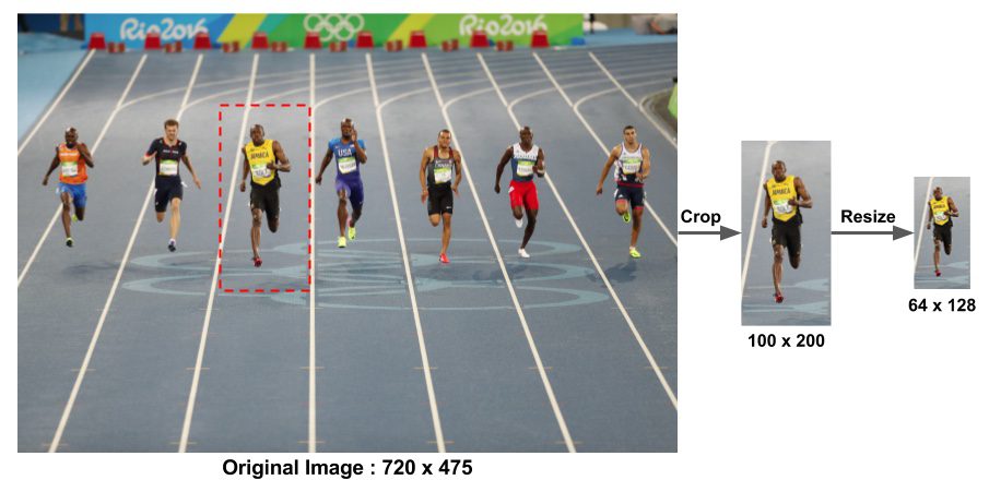
As mentioned earlier HOG feature descriptor used for pedestrian detection is calculated on a 64×128 patch of an image. Of course, an image may be of any size. Typically patches at multiple scales are analyzed at many image locations. The only constraint is that the patches being analyzed have a fixed aspect ratio. In our case, the patches need to have an aspect ratio of 1:2. For example, they can be 100×200, 128×256, or 1000×2000 but not 101×205.
To illustrate this point I have shown a large image of size 720×475. We have selected a patch of size 100×200 for calculating our HOG feature descriptor. This patch is cropped out of an image and resized to 64×128. Now we are ready to calculate the HOG descriptor for this image patch.
The paper by Dalal and Triggs also mentions gamma correction as a preprocessing step, but the performance gains are minor and so we are skipping the step.
Step 2 : Calculate the Gradient Images
To calculate a HOG descriptor, we need to first calculate the horizontal and vertical gradients; after all, we want to calculate the histogram of gradients. This is easily achieved by filtering the image with the following kernels.
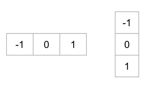
We can also achieve the same results, by using Sobel operator in OpenCV with kernel size 1.
|
1
2
3
4
5
6
7
8
9
|
// C++ gradient calculation.
// Read image
Mat img = imread(
"bolt.png"
);
img.convertTo(img, CV_32F, 1/255.0);
// Calculate gradients gx, gy
Mat gx, gy;
Sobel(img, gx, CV_32F, 1, 0, 1);
Sobel(img, gy, CV_32F, 0, 1, 1);
|
|
1
2
3
4
5
6
7
8
9
|
# Python gradient calculation
# Read image
im
=
cv2.imread(
'bolt.png'
)
im
=
np.float32(im)
/
255.0
# Calculate gradient
gx
=
cv2.Sobel(img, cv2.CV_32F,
1
,
0
, ksize
=
1
)
gy
=
cv2.Sobel(img, cv2.CV_32F,
0
,
1
, ksize
=
1
)
|
Next, we can find the magnitude and direction of gradient using the following formula

If you are using OpenCV, the calculation can be done using the function cartToPolar as shown below.
|
1
2
3
|
// C++ Calculate gradient magnitude and direction (in degrees)
Mat mag, angle;
cartToPolar(gx, gy, mag, angle, 1);
|
The same code in python looks like this.
|
1
2
|
# Python Calculate gradient magnitude and direction ( in degrees )
mag, angle
=
cv2.cartToPolar(gx, gy, angleInDegrees
=
True
)
|
The figure below shows the gradients.
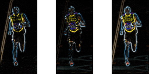 Left : Absolute value of x-gradient. Center : Absolute value of y-gradient. Right : Magnitude of gradient.
Notice, the x-gradient fires on vertical lines and the y-gradient fires on horizontal lines. The magnitude of gradient fires where ever there is a sharp change in intensity. None of them fire when the region is smooth. I have deliberately left out the image showing the direction of gradient because direction shown as an image does not convey much.
The gradient image removed a lot of non-essential information ( e.g. constant colored background ), but highlighted outlines. In other words, you can look at the gradient image and still easily say there is a person in the picture.
At every pixel, the gradient has a magnitude and a direction. For color images, the gradients of the three channels are evaluated ( as shown in the figure above ). The magnitude of gradient at a pixel is the maximum of the magnitude of gradients of the three channels, and the angle is the angle corresponding to the maximum gradient.
Step 3 : Calculate Histogram of Gradients in 8×8 cells
 8×8 cells of HOG. Image is scaled by 4x for display.
In this step, the image is divided into 8×8 cells and a histogram of gradients is calculated for each 8×8 cells.
We will learn about the histograms in a moment, but before we go there let us first understand why we have divided the image into 8×8 cells. One of the important reasons to use a feature descriptor to describe a patch of an image is that it provides a compact representation. An 8×8 image patch contains 8x8x3 = 192 pixel values. The gradient of this patch contains 2 values ( magnitude and direction ) per pixel which adds up to 8x8x2 = 128 numbers. By the end of this section we will see how these 128 numbers are represented using a 9-bin histogram which can be stored as an array of 9 numbers. Not only is the representation more compact, calculating a histogram over a patch makes this represenation more robust to noise. Individual graidents may have noise, but a histogram over 8×8 patch makes the representation much less sensitive to noise.
But why 8×8 patch ? Why not 32×32 ? It is a design choice informed by the scale of features we are looking for. HOG was used for pedestrian detection initially. 8×8 cells in a photo of a pedestrian scaled to 64×128 are big enough to capture interesting features ( e.g. the face, the top of the head etc. ).
The histogram is essentially a vector ( or an array ) of 9 bins ( numbers ) corresponding to angles 0, 20, 40, 60 … 160.
Let us look at one 8×8 patch in the image and see how the gradients look.
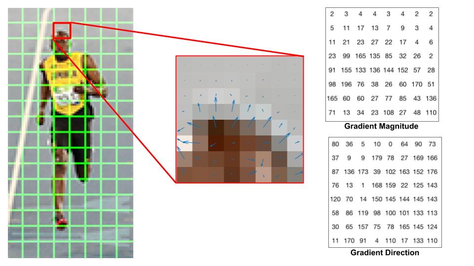 Center : The RGB patch and gradients represented using arrows. Right : The gradients in the same patch represented as numbers
If you are a beginner in computer vision, the image in the center is very informative. It shows the patch of the image overlaid with arrows showing the gradient — the arrow shows the direction of gradient and its length shows the magnitude. Notice how the direction of arrows points to the direction of change in intensity and the magnitude shows how big the difference is.
On the right, we see the raw numbers representing the gradients in the 8×8 cells with one minor difference — the angles are between 0 and 180 degrees instead of 0 to 360 degrees. These are called “unsigned” gradientsbecause a gradient and it’s negative are represented by the same numbers. In other words, a gradient arrow and the one 180 degrees opposite to it are considered the same. But, why not use the 0 – 360 degrees ? Empirically it has been shown that unsigned gradients work better than signed gradients for pedestrian detection. Some implementations of HOG will allow you to specify if you want to use signed gradients.
The next step is to create a histogram of gradients in these 8×8 cells. The histogram contains 9 bins corresponding to angles 0, 20, 40 … 160.
The following figure illustrates the process. We are looking at magnitude and direction of the gradient of the same 8×8 patch as in the previous figure. A bin is selected based on the direction, and the vote ( the value that goes into the bin ) is selected based on the magnitude. Let’s first focus on the pixel encircled in blue. It has an angle ( direction ) of 80 degrees and magnitude of 2. So it adds 2 to the 5th bin. The gradient at the pixel encircled using red has an angle of 10 degrees and magnitude of 4. Since 10 degrees is half way between 0 and 20, the vote by the pixel splits evenly into the two bins.
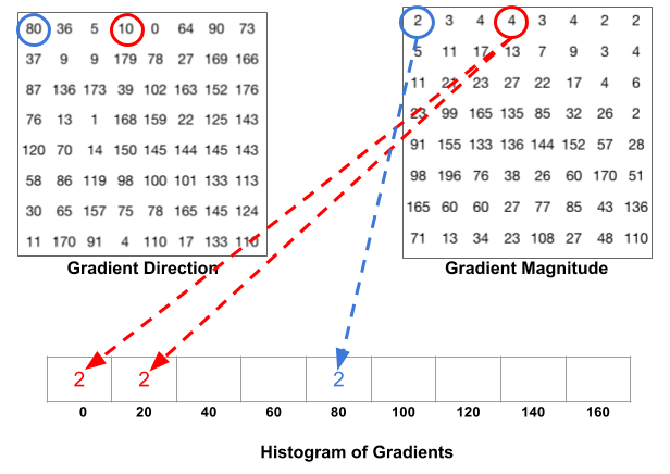
There is one more detail to be aware of. If the angle is greater than 160 degrees, it is between 160 and 180, and we know the angle wraps around making 0 and 180 equivalent. So in the example below, the pixel with angle 165 degrees contributes proportionally to the 0 degree bin and the 160 degree bin.

The contributions of all the pixels in the 8×8 cells are added up to create the 9-bin histogram. For the patch above, it looks like this
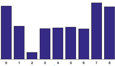
In our representation, the y-axis is 0 degrees. You can see the histogram has a lot of weight near 0 and 180 degrees, which is just another way of saying that in the patch gradients are pointing either up or down.
Step 4 : 16×16 Block Normalization
In the previous step, we created a histogram based on the gradient of the image. Gradients of an image are sensitive to overall lighting. If you make the image darker by dividing all pixel values by 2, the gradient magnitude will change by half, and therefore the histogram values will change by half. Ideally, we want our descriptor to be independent of lighting variations. In other words, we would like to “normalize” the histogram so they are not affected by lighting variations.
Before I explain how the histogram is normalized, let’s see how a vector of length 3 is normalized.
Let’s say we have an RGB color vector [ 128, 64, 32 ]. The length of this vector is  . This is also called the L2 norm of the vector. Dividing each element of this vector by 146.64 gives us a normalized vector [0.87, 0.43, 0.22]. Now consider another vector in which the elements are twice the value of the first vector 2 x [ 128, 64, 32 ] = [ 256, 128, 64 ]. You can work it out yourself to see that normalizing [ 256, 128, 64 ] will result in [0.87, 0.43, 0.22], which is the same as the normalized version of the original RGB vector. You can see that normalizing a vector removes the scale.
Now that we know how to normalize a vector, you may be tempted to think that while calculating HOG you can simply normalize the 9×1 histogram the same way we normalized the 3×1 vector above. It is not a bad idea, but a better idea is to normalize over a bigger sized block of 16×16. A 16×16 block has 4 histograms which can be concatenated to form a 36 x 1 element vector and it can be normalized just the way a 3×1 vector is normalized. The window is then moved by 8 pixels ( see animation ) and a normalized 36×1 vector is calculated over this window and the process is repeated.
Step 5 : Calculate the HOG feature vector
To calculate the final feature vector for the entire image patch, the 36×1 vectors are concatenated into one giant vector. What is the size of this vector ? Let us calculate
- How many positions of the 16×16 blocks do we have ? There are 7 horizontal and 15 vertical positions making a total of 7 x 15 = 105 positions.
- Each 16×16 block is represented by a 36×1 vector. So when we concatenate them all into one gaint vector we obtain a 36×105 = 3780dimensional vector.
Visualizing Histogram of Oriented Gradients
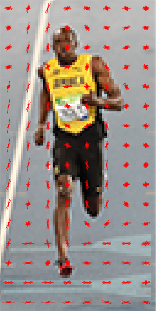
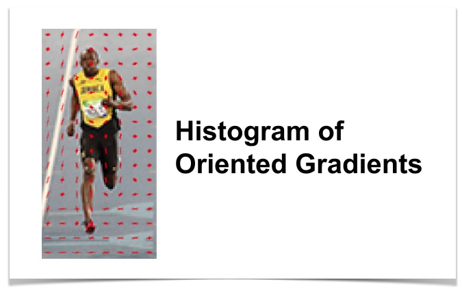
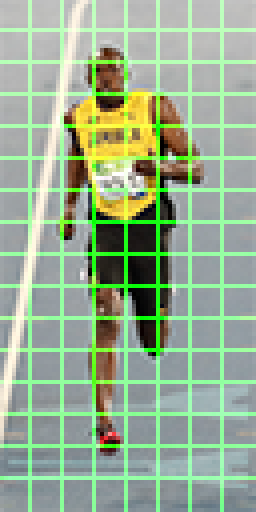
The HOG descriptor of an image patch is usually visualized by plotting the 9×1 normalized histograms in the 8×8 cells. See image on the side. You will notice that dominant direction of the histogram captures the shape of the person, especially around the torso and legs.
Unfortunately, there is no easy way to visualize the HOG descriptor in OpenCV.
Subscribe & Download Code
If you liked this article, please subscribeto our newsletter. You will receive access to the code used in other blog posts and a free Computer Vision Resource guide. In our newsletters, we share OpenCV tutorials and examples written in C++/Python, and Computer Vision and Machine Learning algorithms and news.
中文翻译版:https://www.jianshu.com/p/395f0582c5f7


 3526
3526


 被折叠的 条评论
为什么被折叠?
被折叠的 条评论
为什么被折叠?
 到【灌水乐园】发言


